Enhancement by histogram manipulation

This is our last class activity in image processing. The task is to manipulate the probability distribution function of the image to reveal the details shrouded with shadows. In many cases, modern cameras are very good in resolving details in shadow and highlights as long as the pixels are inside their given dynamic range. Let’s consider the image in Fig 1. I took this photo inside our dark room. In this particular image, I just want to capture the laser beam and the light trails so I lowered my ISO and aperture. My goal is to enhance this photo such that all the details in the dark areas are revealed.

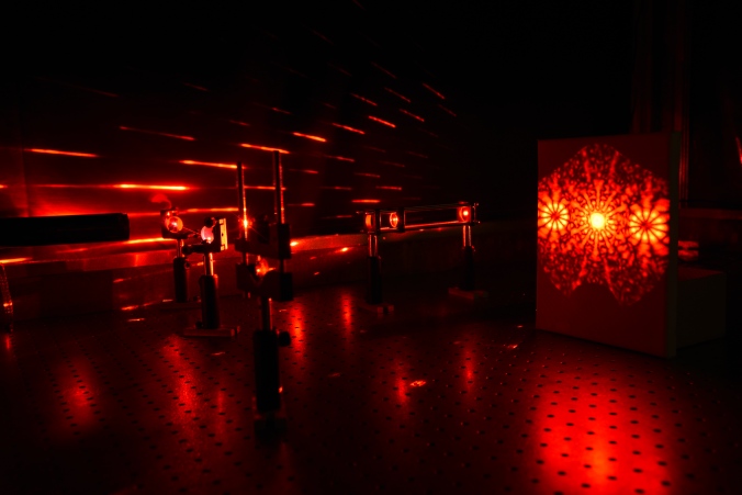
Fig 1. test image.

Let’s deal first with the grayscale version of Fig 1. The first step is to get the histogram of the image and normalized it by the total number of pixels. This normalized histogram is the probability distribution function (PDF) of the image. Next, cumulative sum is performed on the pixel counts to calculate the cumulative distribution function (CDF). The PDF and CDF of Fig are given in Fig 2. Note that the shape of the CDF is similar to logarithmic function.

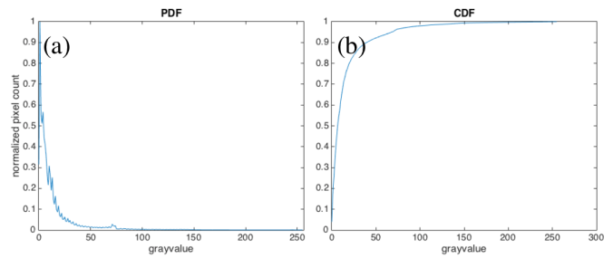
Fig 2 PDF (a) and CDF (b) of Fig 1.

To have a uniform probability distribution, the CDF must be linear in shape. This is the starting point of histogram manipulation part of this activity. For each pixel of the image, I check the grayscale value and its corresponding CDF value. Then, I have to find this CDF value from a pre-made linear CDF and get the  equivalent gray value. This final gray value will be the pixel value of the pixel. When I did this process to my test image, I obtained the image in Fig 3. The new image revealed some interesting details like the laser beam impinging the lens cage system.

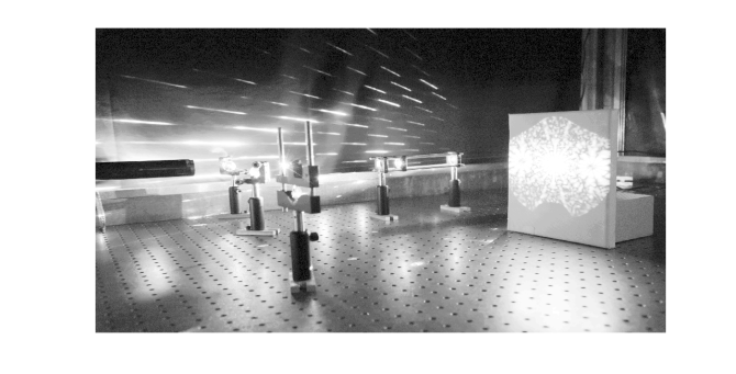
Fig 3. Image with manipulated PDF.

The PDF of the new image (Fig 4.a) is more dispersed than the original PDF. The pixels of the new images are more uniformly distributed  among the highlights, midtones, and shadows of the image. This means that the details of the image are not obscured by the shadows and intense light. The corresponding CDF (Fig 4.b) has a linear profile. This shows that we can enhance the details of an image by using a linear CDF as basis for manipulation.

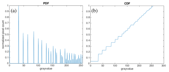
Fig 4. PDF (a) and CDF (b) of the  enhanced image in Fig 3.

What I want to do now is to manipulate the CDF of a colored image. The first step is to normalize the red (R), green (G), and blue (B) channels and thereby transforming them to normalized chromaticity space (r,g, and b). Note that the matrix used for PDF and CDF calculations is only 2D. For colored spaces, we use the matrix  (I) that yields from the sum of 3 color channels. I used another image from my collection to demonstrate the manipulation of colored images. It is an image of Math Building  (Fig 5) which I took from our window. We can see that the image is full of shadows.

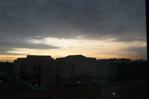
Fig 5. Math building as a test image

After performing the  manipulation of CDF and forcing it to be linear, I was able to reveal the details of the building – windows and  body lines- and the pathway on the grounds between National Institute of Physics and Institute of Mathematics. The enhanced image is in Fig 6.

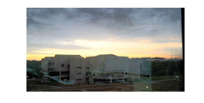
Fig 6. Enhanced image of Math building

Based on my result, I’ve met the goal of this activity.Therefore, my self-evaluation score is  10.

Acknowledgement:

I would like to thank Dr Nathaniel Hermosa for letting me take a photograph of our lab set-up.

Reference:

[1] M. Soriano, AP 186 A10- Enhancement by histogram manipulation. 2016