Basic video processing

Enhancement by histogram manipulation

This is our last class activity in image processing. The task is to manipulate the probability distribution function of the image to reveal the details shrouded with shadows. In many cases, modern cameras are very good in resolving details in shadow and highlights as long as the pixels are inside their given dynamic range. Let’s consider the image in Fig 1. I took this photo inside our dark room. In this particular image, I just want to capture the laser beam and the light trails so I lowered my ISO and aperture. My goal is to enhance this photo such that all the details in the dark areas are revealed.

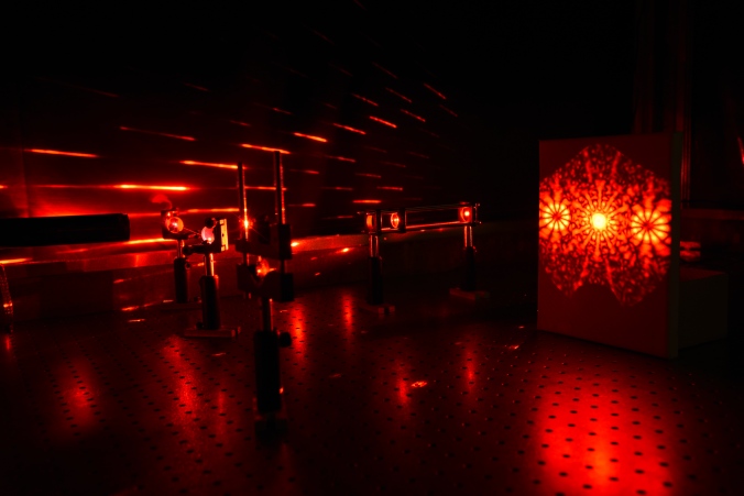
Fig 1. test image.

Let’s deal first with the grayscale version of Fig 1. The first step is to get the histogram of the image and normalized it by the total number of pixels. This normalized histogram is the probability distribution function (PDF) of the image. Next, cumulative sum is performed on the pixel counts to calculate the cumulative distribution function (CDF). The PDF and CDF of Fig are given in Fig 2. Note that the shape of the CDF is similar to logarithmic function.

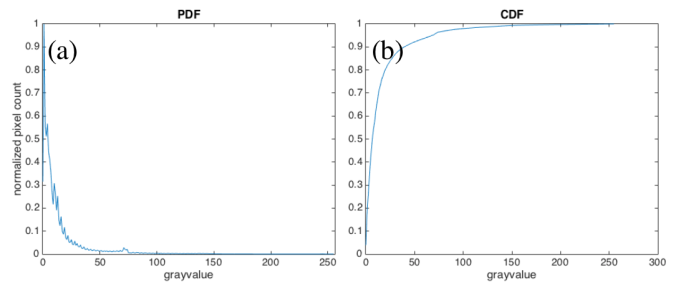
Fig 2 PDF (a) and CDF (b) of Fig 1.

To have a uniform probability distribution, the CDF must be linear in shape. This is the starting point of histogram manipulation part of this activity. For each pixel of the image, I check the grayscale value and its corresponding CDF value. Then, I have to find this CDF value from a pre-made linear CDF and get the  equivalent gray value. This final gray value will be the pixel value of the pixel. When I did this process to my test image, I obtained the image in Fig 3. The new image revealed some interesting details like the laser beam impinging the lens cage system.

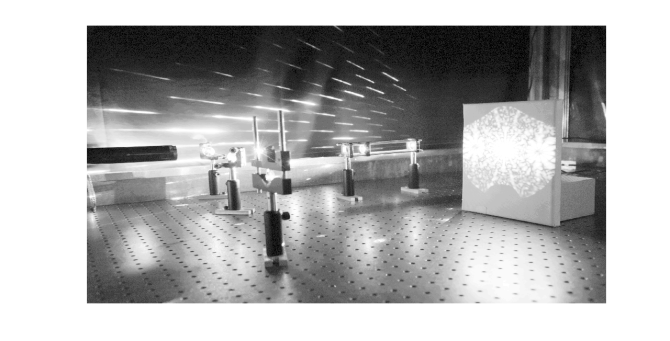
Fig 3. Image with manipulated PDF.

The PDF of the new image (Fig 4.a) is more dispersed than the original PDF. The pixels of the new images are more uniformly distributed  among the highlights, midtones, and shadows of the image. This means that the details of the image are not obscured by the shadows and intense light. The corresponding CDF (Fig 4.b) has a linear profile. This shows that we can enhance the details of an image by using a linear CDF as basis for manipulation.

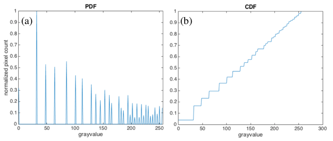
Fig 4. PDF (a) and CDF (b) of the  enhanced image in Fig 3.

What I want to do now is to manipulate the CDF of a colored image. The first step is to normalize the red (R), green (G), and blue (B) channels and thereby transforming them to normalized chromaticity space (r,g, and b). Note that the matrix used for PDF and CDF calculations is only 2D. For colored spaces, we use the matrix  (I) that yields from the sum of 3 color channels. I used another image from my collection to demonstrate the manipulation of colored images. It is an image of Math Building  (Fig 5) which I took from our window. We can see that the image is full of shadows.

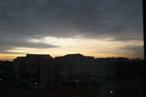
Fig 5. Math building as a test image

After performing the  manipulation of CDF and forcing it to be linear, I was able to reveal the details of the building – windows and  body lines- and the pathway on the grounds between National Institute of Physics and Institute of Mathematics. The enhanced image is in Fig 6.

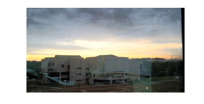
Fig 6. Enhanced image of Math building

Based on my result, I’ve met the goal of this activity.Therefore, my self-evaluation score is  10.

Acknowledgement:

I would like to thank Dr Nathaniel Hermosa for letting me take a photograph of our lab set-up.

Reference:

[1] M. Soriano, AP 186 A10- Enhancement by histogram manipulation. 2016

Playing keynotes by image processing

Fig 1. Original keynote

Fig 2. Keynotes are detected by locating the circles in the image.  Close and open morphological operations are performed to remove the gridlines of the music sheet.

Morphological operations

Today, another image processing technique is waiting for me to discern. I already dealt with image processing in Fourier space and segmentations which I discussed  in my previous blog posts. Now, I will be doing morphological operations. In this technique, binary images are modified based on the operations done with the structuring element.  The operations involved uses set theory to modify the images. They can either shrink, expand, ad fill the gaps of a shape depending on the conditions given between the structuring element and the given object.

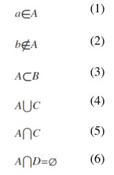
First of all, I want to discuss some set equations that are essential in understanding morphological operations. Consider two large sets A and B which are both collection of objects like letters, numbers, or points. Eq 1-6 are the basic set notions. Eq 1 stands for a is an element of A and this is true if we can find a in set A.  Crossing out the notation signifies negation  so Eq 2 means b is not an element of A. Now, if set A is part of a bigger set B, we can write it as Eq 3. There are  also notations that yields a new set. If we want to get all the elements of sets A and B, we use the union operator in Eq 4. However, if we are only interested in the intersection of two sets, the intersection operator in Eq 5 is the right notation. Finally, the set notation for saying that the new set has no element, like the intersection of A and D in Eq 6, is to equate the relation to null set.

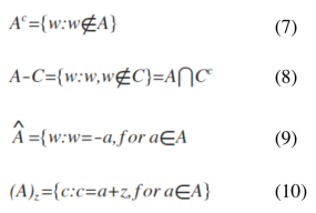
The next things I want to discuss are some arithmetic operations in set theory. Understanding how these are written and interpreted are very essential in performing basic and complex morphological relations. Believe me. It costed me one quiz before realizing it. Eq 7 says that the compliment of A is a set composed of elements (w) which are not in A. The difference (Eq 8) of sets A and C is a set that contains elements (w) that are in A but not in B. The next two equations are usually used when dealing with set of numerical coordinate values. The reflection (Eq 9) of set A is just negated (-)  version of A. For example, if A = {1,2,3,4,5} then the reflection of A is {-1,-2,-3,-4,-5}. The translation (Eq 10) of a set A  is done by adding a constant (z) on its elements.

Finally! Let’s do the fun part. I will now apply these set operations to morphological operations. I this activity, two morphological operations are introduced: dilation (Eq 11) and erosion (Eq 12). Set A is composed of points inside the area of a given shape and set B is called the structuring element. The visualization of each set is a binary image in which each coordinate value that is included in the set has value of 1. The structuring element reshapes the larger set A depending on the conditions given for each operation. It is defined from its center.  To dilate  set A with structuring element B, get the reflection of B first. Then, place the center of the structuring element in each pixel of image of set A and check if the two sets have intersection (translation part). If there is an intersection, mark the current location of the structuring element’s center with 1. After this process is iterated to all the pixels of set A, the result is the dilated image of A. To erode a structure, translate the center of the structuring element (B) to each pixel of image containing the set A and check if the occupied space of the B is a subset of A. Mark the center of B with 1 if this condition is satisfied.

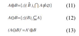
I applied dilation and erosion to various shapes such as square, triangle, hollow square, and cross using structuring elements such as square, vertically and horizontally oriented rectangle, cross and diagonal. The results are in Fig 1 for dilation and Fig 2 for erosion. The topmost rows of both images show the structuring element and the leftmost columns contain the shapes being structured. We can see from the figures that dilation increases the area of the shape while the reverse is observed for erosion. The results also suggests that we need to use a structuring element with the same profile as the shape being structured to preserve the original morphology of the shape.

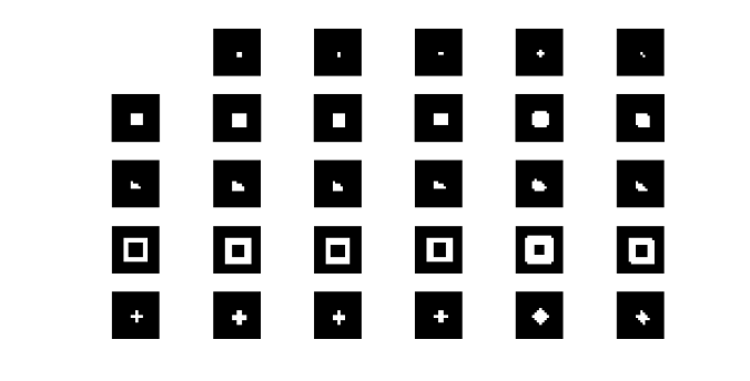
Fig 1. Dilation results. The area covered of the new image for each shape-structuring element pair is greater than the area of the original shape.

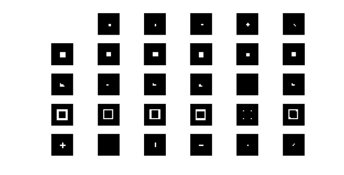
Fig 2. Erosion results. The area covered of the new image for each shape-structuring element pair is smaller than the area of the original shape.

I also did some morphological operations on these shapes with my magnificent  free-hand drawing (haha)  on a graphing paper. The results are pretty much the same. I posted it in Fig 3.

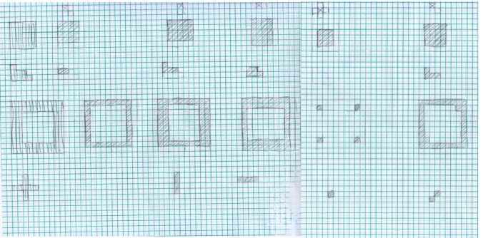
Fig 3. Hand-drawn dilation (top) and erosion (bottom) of square, triangle, hollow square, and cross.

I want to extend further the application of morphological operations to real world situations. This time,  the application is identification of cancer cells. The main problem for isolating cancer cells from the image is the threshold color that segments  cells because it is close to the color of the background. What I want to do is to use the combination of erosion and dilation to clean the segmented image so I can clearly  estimate the area of normal cells. The mean area is used to separate normal cells from cancerous cells. I asked my professor (Dr. Soriano) about why we are isolating the large cells. According to her, cancerous cells are more active than normal cells therefore they are generally bigger.

To do mean area estimation, we are tasked to divide the test image into 256×256 subimages, perform morphological operations to clean up the unnecessary artifacts of thresholding, and estimate the area of the cells. The result of thresholding is in Fig 4. This shows that we need additional steps to clean the image before area estimation.

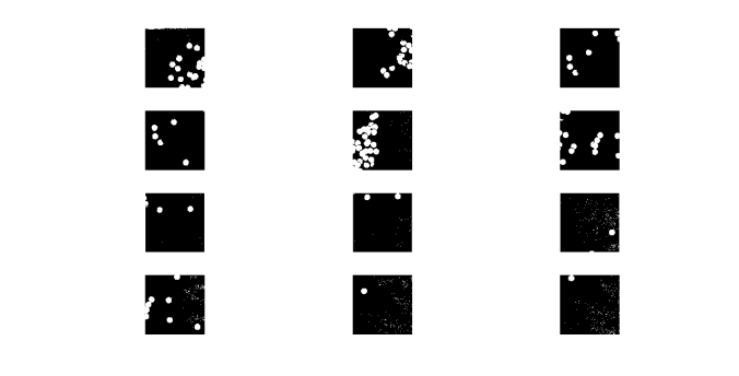
Fig 4.  After thresholding, artifacts are found in some subimages. These must be removed before proceeding to area estimation.

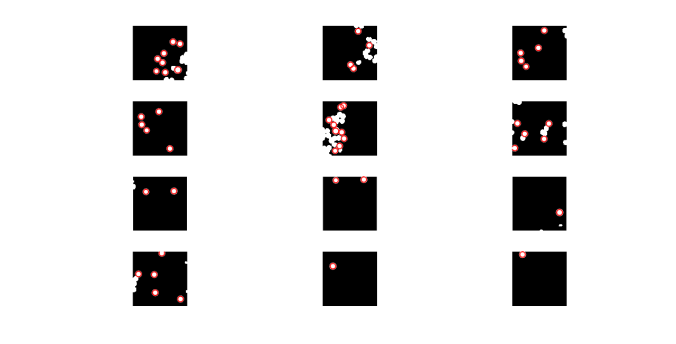
Fig 5. Subimages after close-open morphological operation was performed. The circles with red outlines are used to estimate the mean area.

After performing morphological operations to clean the images and area estimation, the mean area obtained was 528 and the standard deviation was 42. This was used to isolate the cancerous cells to normal cells. We were given an image with cancer cells. I performed the morphological operation I used in the segmentation part and then I searched the circles with areas greater than the mean area plus the standard deviation. My results are in Fig 6.

Fig 6. Image with identified cancer cells (outlined with red).

Finally I’m done! This task is both rewarding and exhausting. I think I clearly provided the necessary steps to perform this tasks and obtained good results. For this, my self rating is 10.

References:

[1] M. Soriano, AP 186 A8- Morphological operations 2014. 2016

[2] “GpuArray.” Morphologically Close Image – MATLAB Imclose. N.p., n.d. Web. 06 Dec. 2016.

[3] “GpuArray.” Morphologically Open Image – MATLAB Imopen. N.p., n.d. Web. 06 Dec. 2016.

Image segmentation

My next project is about image segmentation. From the word itself, this task aims to isolate an object from an image based on the object color. For grayscale images, the process is simple. The only step that will shake your brain is getting the histogram of pixel values of the image. This is followed by checking the threshold (lower and upper limit) values of your region  of interest. The last step is binarizing the whole image in such a way that all pixels inside the lower and upper threshold have values equal to 1 and the other pixels outside this are set to 0. To do the final step, use a boolean operator to make the binarized image. Let’s consider the image in Fig 1. As I said before, the hardest part for this case is plotting the histogram. Luckily, Ma’am Soriano (thank you!) gave us the code. That code is so important because it is the main bulk of image processing techniques that utilize histograms. I’ll leave it Fig 2 for future references. Moving on, the histogram of the image in Fig 1 is presented in Fig 3.

Fig 1. Sample grayscale image

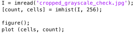
Fig 2. Histogram code

My main interest in Fig 1 is the texts and I want to segment it from the white background. In the histogram (Fig 3), we can see that the pixel values are dominated by the bright spaces in the sample image. What I want to do is to set the pixel values of the background to zero and this time, the boolean operator will do its part.

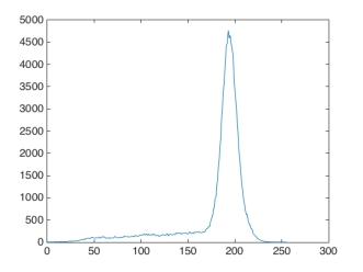
Fig 3. Histogram of Fig 1.

Just perform the code snippet- Im = I

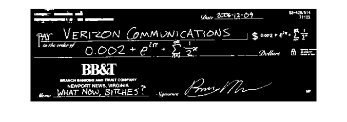
Fig 4. Binarized image of Fig1.

In segmenting colored objects from the image, there are two possible methods: parametric and non-parametric segmentation. I  deal mainly with the histogram of the whole image and look which part of it where the color of our object most probably belongs. Therefore, the first step is to crop some portion of our object and this is called  the region of interest (ROI). Then, each color channel (R,G, and B) is normalized by dividing the whole matrix by the sum of the three channels (R+G+B). This will result to normalized color channels (r, g, and b). Note that normalized blue color channel is just the difference of 1 and the sum of the remaining two normalized color channels (r+g). Therefore,  the number of independent color channels is reduced from 3 to 2. The  succeeding processes for each method mentioned earlier will branch out from this point.

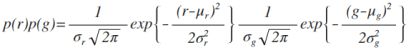
For the parametric segmentation, we have to calculate the mean and standard deviation of red and green normalized color channels and assume that the probability distribution function of eacf color follows the gaussian distribution (Eq 1). My test image contains numerous spheres with different colors and my ROI is the red sphere. I displayed it in Fig 5.

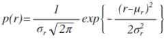   (1)

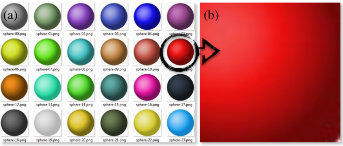
   Fig 5. Test image (a) and the chosen ROI (b)

To check if the color of each pixel belongs to the color of the ROI, just implement the joint probability of red and green colors (p(r)p(g)). This will tag a value to one pixel depending on the probability that the color belongs to the ROI. The result (Fig 6.b) is an image in which only the ROI pixels have higher values compared to the other pixels with different color. Therefore, the object is said to be segmented.

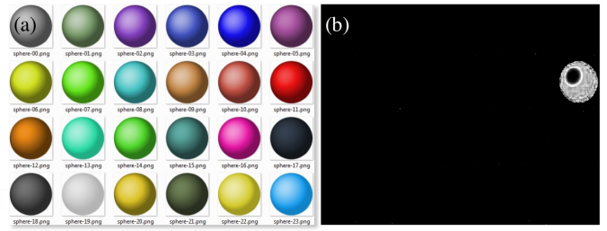
Fig 6. Test image (a) and segmented image using parametric segmentation(b)

The parametric equation I use to segment is given in Eq 2.

                       (2)

The next and final segmentation utilizes the histograms of the ROI and the test image directly and no further calculation is needed. Sounds good right? The process is more direct and lessens the trouble of calculating the mean and standard deviation but for me, the algorithm of this technique is more challenging to construct. Histogram construction is not as intuitive as it seems but more rewarding if you finally understand how it is done. It feels like you are now a true histogram maker.

Following from the normalization step, I need to put all the color values of red and green normalized color channels into one long array. To do this, the pixel values must be binned such that the first half of the bins accommodates the red pixel values while the other half is occupied by the green pixel values. Now, I have to deal with the histogram construction again and plotting it with three color channels is not intuitive. Again, the code for this is given in Fig 7. The for loops counts the number of pixels that falls on a given color value.

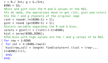
Fig 7. Code snippet for binning of colors.

The next thing to do is to recover the histogram coordinates of the ROI and convert it into the color values. Separate them using the technique of multiplying and adding scheme before. All pixels of the image are given with grayvalues depending on the probability of its initial color which is based on the histogram of the ROI.

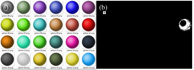
Fig 8. Test image (a) and segmented image using non-parametric segmentation (b)

Both methods are able segment the ROI from the whole image. The direct advantage of non-parametric is the fact that no calculation of mean and standard deviation is needed. It uses the histogram directly to separate the ROI from the original image. This can save some time if you are dealing with hundreds of images to segment with.

I’m done! I was able to demonstrate both methods clearly. I was successful in segmenting a  colored ROI from the original image. This activity took me a lot of time and effort to finish. Therefore, I will give my self a 10.

References:

[1] M. Soriano, AP 186  A7 – Image Segmentation. 2016.

[2]https://www.google.com.ph/urlsa=i&rct=j&q=&esrc=s&source=images&cd=&ved=0ahUKEwiQur6EruLQAhWBtI8KHUsDAuMQjxwIAw&url=http%3A%2F%2Fopengameart.org%2Fcontent%2Fcoloredspheres&bvm=bv.140496471,d.c2I&psig=AFQjCNFt8fmPmylbMlZfRelwvuArEy0Vhg&ust=1481209637460827