Basic video processing

Enhancement by histogram manipulation

This is our last class activity in image processing. The task is to manipulate the probability distribution function of the image to reveal the details shrouded with shadows. In many cases, modern cameras are very good in resolving details in shadow and highlights as long as the pixels are inside their given dynamic range. Let’s consider the image in Fig 1. I took this photo inside our dark room. In this particular image, I just want to capture the laser beam and the light trails so I lowered my ISO and aperture. My goal is to enhance this photo such that all the details in the dark areas are revealed.

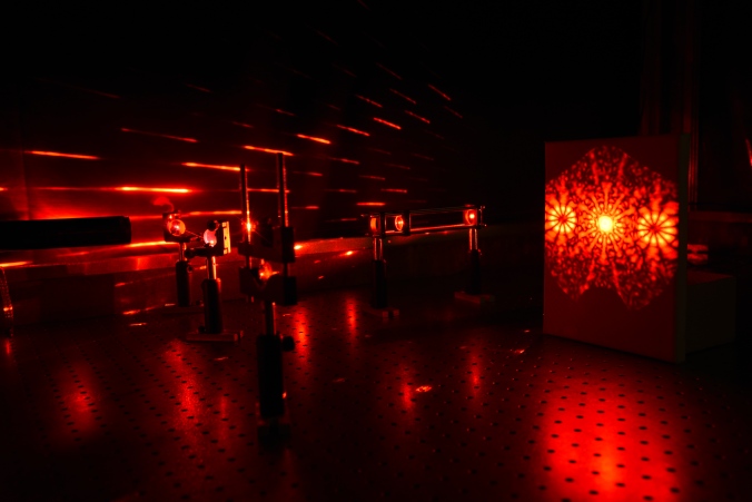
Fig 1. test image.

Let’s deal first with the grayscale version of Fig 1. The first step is to get the histogram of the image and normalized it by the total number of pixels. This normalized histogram is the probability distribution function (PDF) of the image. Next, cumulative sum is performed on the pixel counts to calculate the cumulative distribution function (CDF). The PDF and CDF of Fig are given in Fig 2. Note that the shape of the CDF is similar to logarithmic function.

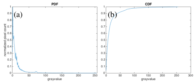
Fig 2 PDF (a) and CDF (b) of Fig 1.

To have a uniform probability distribution, the CDF must be linear in shape. This is the starting point of histogram manipulation part of this activity. For each pixel of the image, I check the grayscale value and its corresponding CDF value. Then, I have to find this CDF value from a pre-made linear CDF and get the  equivalent gray value. This final gray value will be the pixel value of the pixel. When I did this process to my test image, I obtained the image in Fig 3. The new image revealed some interesting details like the laser beam impinging the lens cage system.

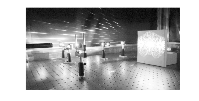
Fig 3. Image with manipulated PDF.

The PDF of the new image (Fig 4.a) is more dispersed than the original PDF. The pixels of the new images are more uniformly distributed  among the highlights, midtones, and shadows of the image. This means that the details of the image are not obscured by the shadows and intense light. The corresponding CDF (Fig 4.b) has a linear profile. This shows that we can enhance the details of an image by using a linear CDF as basis for manipulation.

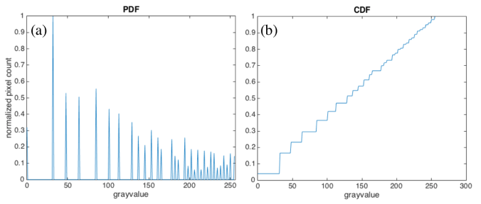
Fig 4. PDF (a) and CDF (b) of the  enhanced image in Fig 3.

What I want to do now is to manipulate the CDF of a colored image. The first step is to normalize the red (R), green (G), and blue (B) channels and thereby transforming them to normalized chromaticity space (r,g, and b). Note that the matrix used for PDF and CDF calculations is only 2D. For colored spaces, we use the matrix  (I) that yields from the sum of 3 color channels. I used another image from my collection to demonstrate the manipulation of colored images. It is an image of Math Building  (Fig 5) which I took from our window. We can see that the image is full of shadows.

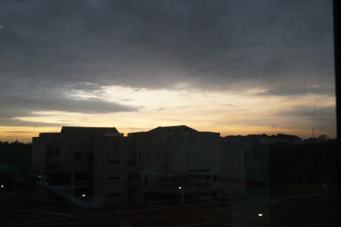
Fig 5. Math building as a test image

After performing the  manipulation of CDF and forcing it to be linear, I was able to reveal the details of the building – windows and  body lines- and the pathway on the grounds between National Institute of Physics and Institute of Mathematics. The enhanced image is in Fig 6.

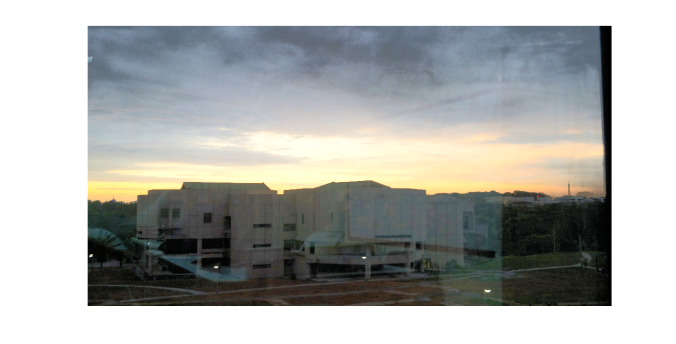
Fig 6. Enhanced image of Math building

Based on my result, I’ve met the goal of this activity.Therefore, my self-evaluation score is  10.

Acknowledgement:

I would like to thank Dr Nathaniel Hermosa for letting me take a photograph of our lab set-up.

Reference:

[1] M. Soriano, AP 186 A10- Enhancement by histogram manipulation. 2016

Playing keynotes by image processing

Fig 1. Original keynote

Fig 2. Keynotes are detected by locating the circles in the image.  Close and open morphological operations are performed to remove the gridlines of the music sheet.

Morphological operations

Today, another image processing technique is waiting for me to discern. I already dealt with image processing in Fourier space and segmentations which I discussed  in my previous blog posts. Now, I will be doing morphological operations. In this technique, binary images are modified based on the operations done with the structuring element.  The operations involved uses set theory to modify the images. They can either shrink, expand, ad fill the gaps of a shape depending on the conditions given between the structuring element and the given object.

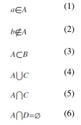
First of all, I want to discuss some set equations that are essential in understanding morphological operations. Consider two large sets A and B which are both collection of objects like letters, numbers, or points. Eq 1-6 are the basic set notions. Eq 1 stands for a is an element of A and this is true if we can find a in set A.  Crossing out the notation signifies negation  so Eq 2 means b is not an element of A. Now, if set A is part of a bigger set B, we can write it as Eq 3. There are  also notations that yields a new set. If we want to get all the elements of sets A and B, we use the union operator in Eq 4. However, if we are only interested in the intersection of two sets, the intersection operator in Eq 5 is the right notation. Finally, the set notation for saying that the new set has no element, like the intersection of A and D in Eq 6, is to equate the relation to null set.

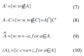
The next things I want to discuss are some arithmetic operations in set theory. Understanding how these are written and interpreted are very essential in performing basic and complex morphological relations. Believe me. It costed me one quiz before realizing it. Eq 7 says that the compliment of A is a set composed of elements (w) which are not in A. The difference (Eq 8) of sets A and C is a set that contains elements (w) that are in A but not in B. The next two equations are usually used when dealing with set of numerical coordinate values. The reflection (Eq 9) of set A is just negated (-)  version of A. For example, if A = {1,2,3,4,5} then the reflection of A is {-1,-2,-3,-4,-5}. The translation (Eq 10) of a set A  is done by adding a constant (z) on its elements.

Finally! Let’s do the fun part. I will now apply these set operations to morphological operations. I this activity, two morphological operations are introduced: dilation (Eq 11) and erosion (Eq 12). Set A is composed of points inside the area of a given shape and set B is called the structuring element. The visualization of each set is a binary image in which each coordinate value that is included in the set has value of 1. The structuring element reshapes the larger set A depending on the conditions given for each operation. It is defined from its center.  To dilate  set A with structuring element B, get the reflection of B first. Then, place the center of the structuring element in each pixel of image of set A and check if the two sets have intersection (translation part). If there is an intersection, mark the current location of the structuring element’s center with 1. After this process is iterated to all the pixels of set A, the result is the dilated image of A. To erode a structure, translate the center of the structuring element (B) to each pixel of image containing the set A and check if the occupied space of the B is a subset of A. Mark the center of B with 1 if this condition is satisfied.

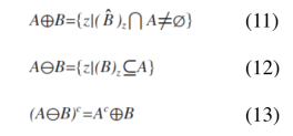
I applied dilation and erosion to various shapes such as square, triangle, hollow square, and cross using structuring elements such as square, vertically and horizontally oriented rectangle, cross and diagonal. The results are in Fig 1 for dilation and Fig 2 for erosion. The topmost rows of both images show the structuring element and the leftmost columns contain the shapes being structured. We can see from the figures that dilation increases the area of the shape while the reverse is observed for erosion. The results also suggests that we need to use a structuring element with the same profile as the shape being structured to preserve the original morphology of the shape.

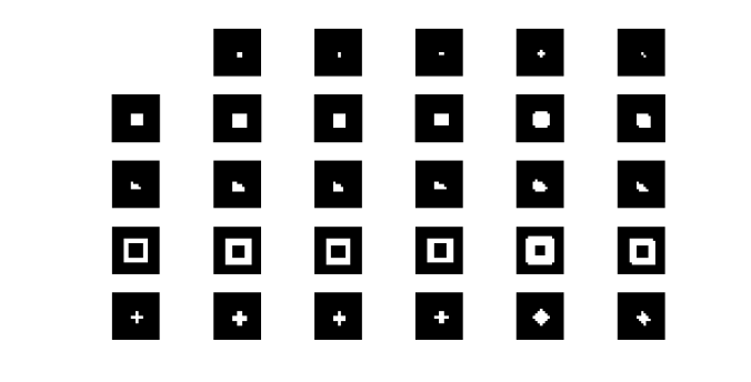
Fig 1. Dilation results. The area covered of the new image for each shape-structuring element pair is greater than the area of the original shape.

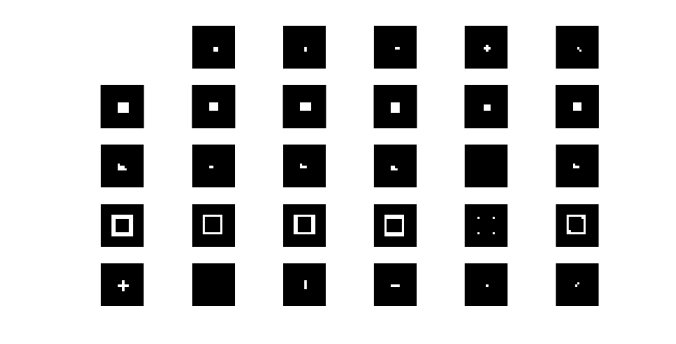
Fig 2. Erosion results. The area covered of the new image for each shape-structuring element pair is smaller than the area of the original shape.

I also did some morphological operations on these shapes with my magnificent  free-hand drawing (haha)  on a graphing paper. The results are pretty much the same. I posted it in Fig 3.

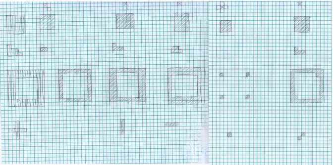
Fig 3. Hand-drawn dilation (top) and erosion (bottom) of square, triangle, hollow square, and cross.

I want to extend further the application of morphological operations to real world situations. This time,  the application is identification of cancer cells. The main problem for isolating cancer cells from the image is the threshold color that segments  cells because it is close to the color of the background. What I want to do is to use the combination of erosion and dilation to clean the segmented image so I can clearly  estimate the area of normal cells. The mean area is used to separate normal cells from cancerous cells. I asked my professor (Dr. Soriano) about why we are isolating the large cells. According to her, cancerous cells are more active than normal cells therefore they are generally bigger.

To do mean area estimation, we are tasked to divide the test image into 256×256 subimages, perform morphological operations to clean up the unnecessary artifacts of thresholding, and estimate the area of the cells. The result of thresholding is in Fig 4. This shows that we need additional steps to clean the image before area estimation.

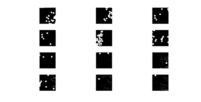
Fig 4.  After thresholding, artifacts are found in some subimages. These must be removed before proceeding to area estimation.

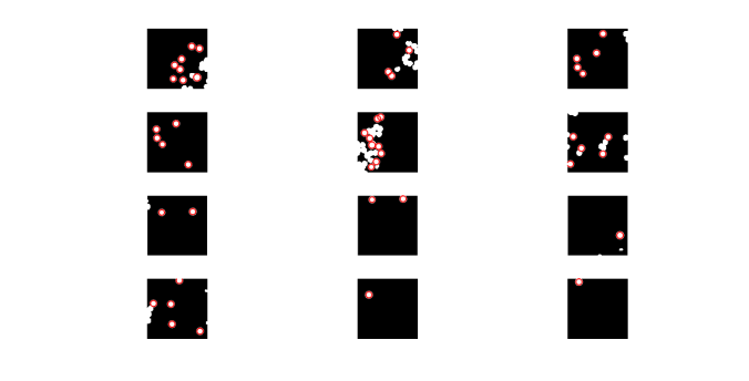
Fig 5. Subimages after close-open morphological operation was performed. The circles with red outlines are used to estimate the mean area.

After performing morphological operations to clean the images and area estimation, the mean area obtained was 528 and the standard deviation was 42. This was used to isolate the cancerous cells to normal cells. We were given an image with cancer cells. I performed the morphological operation I used in the segmentation part and then I searched the circles with areas greater than the mean area plus the standard deviation. My results are in Fig 6.

Fig 6. Image with identified cancer cells (outlined with red).

Finally I’m done! This task is both rewarding and exhausting. I think I clearly provided the necessary steps to perform this tasks and obtained good results. For this, my self rating is 10.

References:

[1] M. Soriano, AP 186 A8- Morphological operations 2014. 2016

[2] “GpuArray.” Morphologically Close Image – MATLAB Imclose. N.p., n.d. Web. 06 Dec. 2016.

[3] “GpuArray.” Morphologically Open Image – MATLAB Imopen. N.p., n.d. Web. 06 Dec. 2016.

Image segmentation

My next project is about image segmentation. From the word itself, this task aims to isolate an object from an image based on the object color. For grayscale images, the process is simple. The only step that will shake your brain is getting the histogram of pixel values of the image. This is followed by checking the threshold (lower and upper limit) values of your region  of interest. The last step is binarizing the whole image in such a way that all pixels inside the lower and upper threshold have values equal to 1 and the other pixels outside this are set to 0. To do the final step, use a boolean operator to make the binarized image. Let’s consider the image in Fig 1. As I said before, the hardest part for this case is plotting the histogram. Luckily, Ma’am Soriano (thank you!) gave us the code. That code is so important because it is the main bulk of image processing techniques that utilize histograms. I’ll leave it Fig 2 for future references. Moving on, the histogram of the image in Fig 1 is presented in Fig 3.

Fig 1. Sample grayscale image

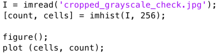
Fig 2. Histogram code

My main interest in Fig 1 is the texts and I want to segment it from the white background. In the histogram (Fig 3), we can see that the pixel values are dominated by the bright spaces in the sample image. What I want to do is to set the pixel values of the background to zero and this time, the boolean operator will do its part.

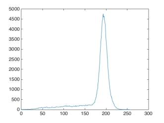
Fig 3. Histogram of Fig 1.

Just perform the code snippet- Im = I

Fig 4. Binarized image of Fig1.

In segmenting colored objects from the image, there are two possible methods: parametric and non-parametric segmentation. I  deal mainly with the histogram of the whole image and look which part of it where the color of our object most probably belongs. Therefore, the first step is to crop some portion of our object and this is called  the region of interest (ROI). Then, each color channel (R,G, and B) is normalized by dividing the whole matrix by the sum of the three channels (R+G+B). This will result to normalized color channels (r, g, and b). Note that normalized blue color channel is just the difference of 1 and the sum of the remaining two normalized color channels (r+g). Therefore,  the number of independent color channels is reduced from 3 to 2. The  succeeding processes for each method mentioned earlier will branch out from this point.

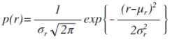
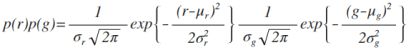
For the parametric segmentation, we have to calculate the mean and standard deviation of red and green normalized color channels and assume that the probability distribution function of eacf color follows the gaussian distribution (Eq 1). My test image contains numerous spheres with different colors and my ROI is the red sphere. I displayed it in Fig 5.

   (1)

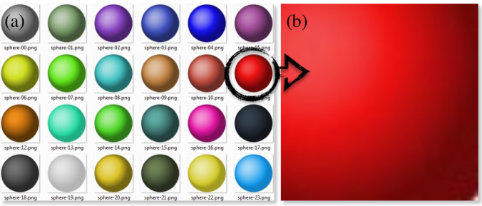
   Fig 5. Test image (a) and the chosen ROI (b)

To check if the color of each pixel belongs to the color of the ROI, just implement the joint probability of red and green colors (p(r)p(g)). This will tag a value to one pixel depending on the probability that the color belongs to the ROI. The result (Fig 6.b) is an image in which only the ROI pixels have higher values compared to the other pixels with different color. Therefore, the object is said to be segmented.

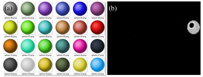
Fig 6. Test image (a) and segmented image using parametric segmentation(b)

The parametric equation I use to segment is given in Eq 2.

                       (2)

The next and final segmentation utilizes the histograms of the ROI and the test image directly and no further calculation is needed. Sounds good right? The process is more direct and lessens the trouble of calculating the mean and standard deviation but for me, the algorithm of this technique is more challenging to construct. Histogram construction is not as intuitive as it seems but more rewarding if you finally understand how it is done. It feels like you are now a true histogram maker.

Following from the normalization step, I need to put all the color values of red and green normalized color channels into one long array. To do this, the pixel values must be binned such that the first half of the bins accommodates the red pixel values while the other half is occupied by the green pixel values. Now, I have to deal with the histogram construction again and plotting it with three color channels is not intuitive. Again, the code for this is given in Fig 7. The for loops counts the number of pixels that falls on a given color value.

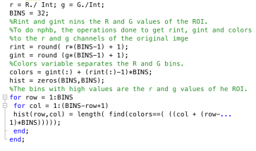
Fig 7. Code snippet for binning of colors.

The next thing to do is to recover the histogram coordinates of the ROI and convert it into the color values. Separate them using the technique of multiplying and adding scheme before. All pixels of the image are given with grayvalues depending on the probability of its initial color which is based on the histogram of the ROI.

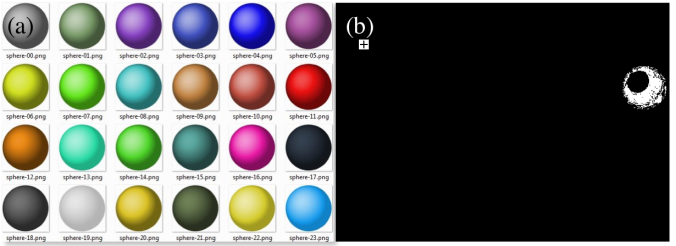
Fig 8. Test image (a) and segmented image using non-parametric segmentation (b)

Both methods are able segment the ROI from the whole image. The direct advantage of non-parametric is the fact that no calculation of mean and standard deviation is needed. It uses the histogram directly to separate the ROI from the original image. This can save some time if you are dealing with hundreds of images to segment with.

I’m done! I was able to demonstrate both methods clearly. I was successful in segmenting a  colored ROI from the original image. This activity took me a lot of time and effort to finish. Therefore, I will give my self a 10.

References:

[1] M. Soriano, AP 186  A7 – Image Segmentation. 2016.

[2]https://www.google.com.ph/urlsa=i&rct=j&q=&esrc=s&source=images&cd=&ved=0ahUKEwiQur6EruLQAhWBtI8KHUsDAuMQjxwIAw&url=http%3A%2F%2Fopengameart.org%2Fcontent%2Fcoloredspheres&bvm=bv.140496471,d.c2I&psig=AFQjCNFt8fmPmylbMlZfRelwvuArEy0Vhg&ust=1481209637460827

Properties and Applications of 2D Fourier Transform

This activity is about numerical signal filtering in Fourier space. The the goal is to work on the Fourier transform of some images, filter out the unnecessary frequency signals and then render it. Before that, we explore first two properties of 2D Fourier transform: anamorphism and rotation property.

First, I want to talk about anamorphism. The dimension of Fourier space is the inverse of the dimension of the image. This tells that what is large in image space will be small in Fourier space. This property is called anamorphism. Consider now the tall rectangle in (a) of figure 1. It has wider extent along the vertical (y) axis compared to its counterpart in horizontal (x) axis. Therefore, its Fourier transform, which is a sinc function, is wider along the x-axis compared to the y-axis as shown in figure 1b. However, when the wide rectangle is transformed, the result is a sinc function that is wider along the y-axis.

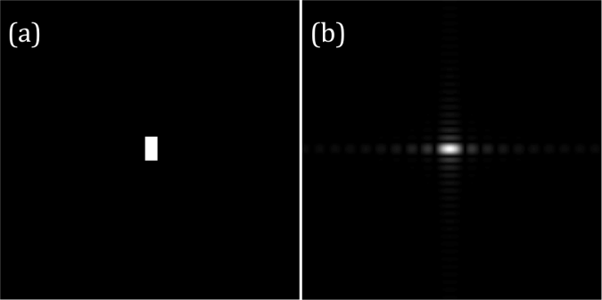
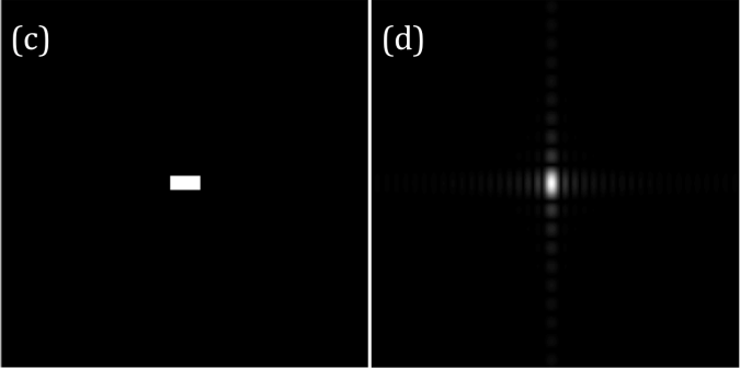
Figure 1. Tall (a) and wide (c) rectangles and their Fourier transforms (b) and (d) respectively.

To demonstrate anamorphism to other patterns, let’s have a look on the Fourier transforms of two dots with different spacing in figures 2. The Fourier transform for this case is composed of vertical bars. It is clearly seen that the as the dots become farther away from each other, the spacing of the bars in Fourier space also increases.

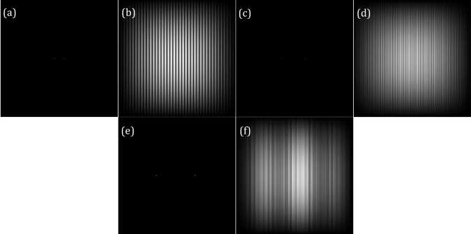
       Figure 2 The set of two dots in (a), (c) and (e) with different separation distances and their Fourier transforms in (b), (d), and (f) respectively.

            For the rotation property of Fourier transform, consider now a rotated sinusoid or corrugated roof about the origin. The sinusoid is z = sin(2πfy) with frequency is f = 4 Hz and its Fourier transform is composed of two Dirac deltas located on its frequency as shown in figures 3a and 3b. I also increased the frequency to 20 Hz and 30 Hz. As expected, the Dirac deltas become farther and farther apart as the frequency is increased (refer to figures 3c-e). Images has no negative values therefore to simulate a sinusoid captured by a camera, a constant bias (also known as DC signal) must be added to it. This added value has no frequency so The Fourier transform of the simulated image has a large peak on f = 0. This DC signal obscures the sinusoid signal for it has larger magnitude which is why only the central peek is visible in figure 3g. Therefore, to recover the true signal, this DC signal should be removed in Fourier space. The bias can also be a non-constant function such as another sinusoid. If this bias is added the original signal, the result is in figure 6.Its Fourier transform, However, it has 4 peaks (refer to figure 6b) pinpointing the frequencies of the original signal and the bias. To recover the original signal, the frequency of the bias must be removed in Fourier space before rendering back to the original space of the image.

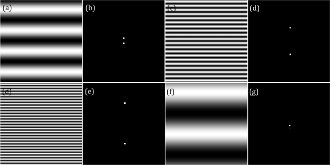
Figure 3 Sinusoids with f = 4 Hz (a), 20 Hz (c) and 30 Hz (d) and their Fourier transforms (b), (d) and (e). The biased sinusoid and its Fourier transform are given , ,however, in (f) and (g).

Moving on, I rotated the sinusiod by modifying its phase term such that new function is z = sin(2πf(ysin(θ) + xcos(θ))) where θ is the rotation angle with respect to the x-axis. The sinusoid is rotated by θ = 45, 90, and 135 degrees. As a result, the Dirac deltas in Fourier space rotates as well in the same direction of θ. The rotated sinusoids and their Fourier transforms were given in figure 4.

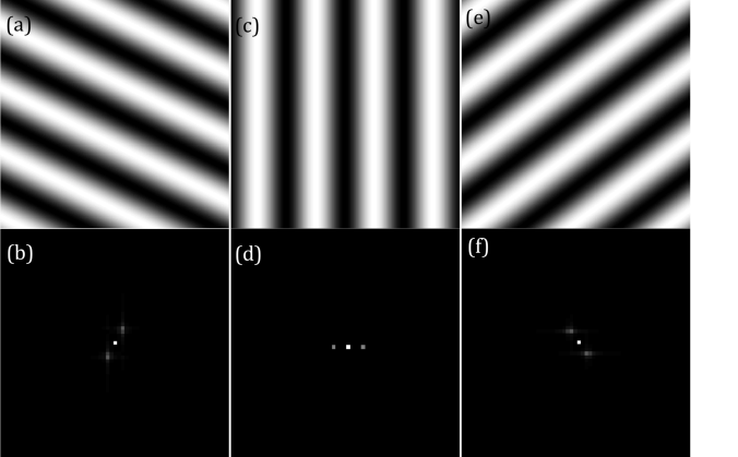
Figure 4 Rotated sinusoids-(a), (c) and (e)- and their Fourier transforms in (b), (d) and (f).

We now investigate the transform a sinusoid multiplied with another sinusoid. Their frequencies are 4 Hz and 8 Hz respectively and the new function is u0 = sin(2π4y).*sin(2π8x). The results were presented in figure 5. The 4 off-centered peaks in Fourier space are located in points (4,8), (-4,8), (4,-8) ,and (-4,-8). Therefore, the multiplied sinusoid modulated such that their frequencies pair up forming a new set.

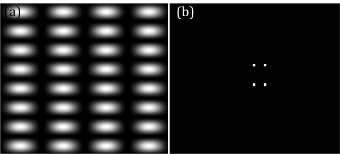
Figure 5 Product of two sinusoids (a) and their Fourier transform (b).

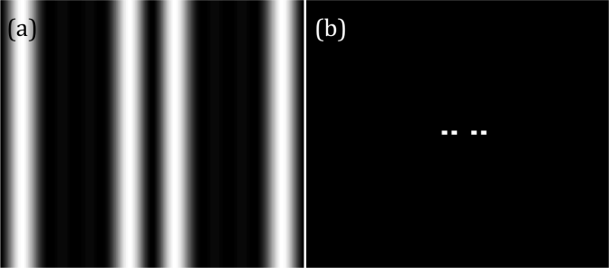
Figure 6 Sum of two sinusoids (a) and their Fourier transform (b).

Before we proceed to the image processing techniques, let’s observe first Dirac delta function and its Fourier transform. Dirac delta function is simulated by assigning one pixel to be one and the rest have 0 value. When to two Dirac deltas equidistant about the origin and placed along the x-axis are transformed in Fourier space, the result is composed of equally spaced vertical bars. When the Dirac deltas are replaced by rectangular, circular or Gaussian function, their Fourier transforms have undulations inside the envelopes which are the transforms of these objects(i.e. F{square aperture} = sinc function) as shown in figure7. However, as their dimensions become smaller, their Fourier transforms are approximately the same as the Dirac deltas’.


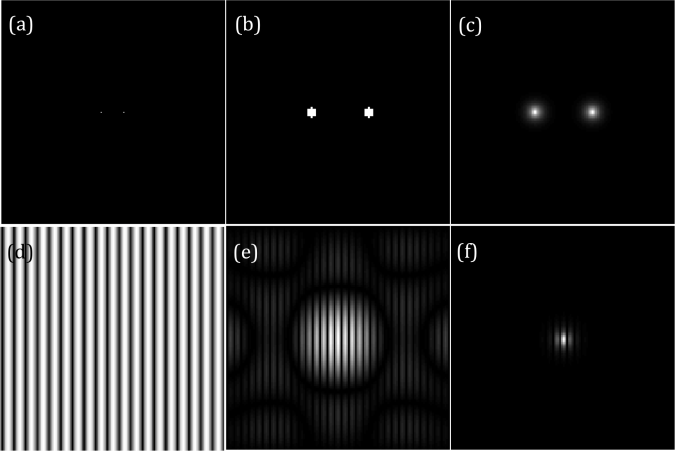
Figure 7 The Fourier transforms of 2 dots (a), 2 circles (b) and 2 gaussian apertures (c) are given in (d), (e) and (f) respectively.

Another exciting fact about Dirac delta is the fact that it brings the function convolved to it on its present location. I used a random 3×3 pattern to demonstrate it. It can be seen in figure 8. that the convolution of the Dirac deltas with the pattern resulted to image with miniature version of the pattern on the location of the Dirac deltas.

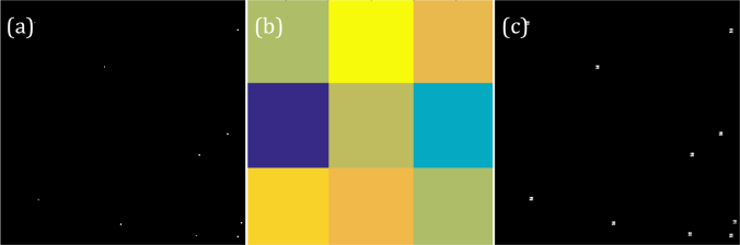
Figure 8. The convolution of Dirac deltas (a) and random pattern(b) results to (c).

Finally, the Fourier transform of an array of Dirac deltas. The contribution of the Dirac deltas along the y axis modulates the Fourier transforms of Dirac deltas lining up the x axis and forming an array of sinc functions and it is shown in figure 9. The number of bright peaks in Fourier space is equal to the number of Dirac deltas.

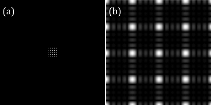
Figure 9. A 5×5 matrix of Dirac Deltas (a) and its Fourier transform (b)

After a long discussion about the properties of Fourier transform, we are ready to do dome image processing using this as a tool. The first image to be processed is from the Lunar Orbiter. It is a panorama with evident bright lines between each stitched frame. We want to eliminate these lines to render a smooth image. Notice that these horizontal lines occur periodically in the image. Therefore, its Fourier transform is composed of points along the y-axis. I filtered it out by blocking the signal along the y-axis of its transform and the result is a smooth picture as shown in figure 10c

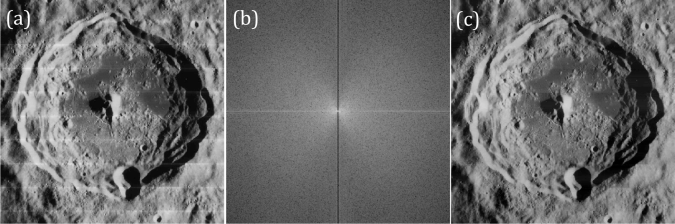
Figure 10. Image from Lunar orbiter (a), its filtered Fourier transform (b) and the rendered image after filtering (c).

The next images is a picture of fingerprint. What we want is to enhance the contrast of the ridges of the patterns. The image has tightly spaced periodic patterns so the Fourier transform of this has more signal on higher frequencies. Also, the periodic lines are oblique so I expect that the frequency signals traces a round path. I filtered out the signals with lower frequencies except the DC term. The ridges become more pronounced than the previous image and it was shown in figure 11.

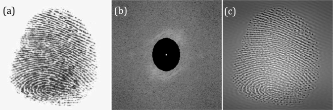
Figure11. Image of fingerprint (a), its filtered Fourier transform (b) and the rendered image after filtering (c).

For the last part we were tasked to obtain the canvass weave of a painting. The weave pattern is evident from the painting itself. It is a rotated periodic pattern which seems to be sinusoids that are either superimposed or multiplied to each other. Knowing this, I designed a filter that extracts the peaks corresponding to these sinusoids in Fourier space and projected it back to original plane. The result is an image of just the canvass weave. The original image of painting, its Fourier transform ,and its canvass weave are shown in figure 12

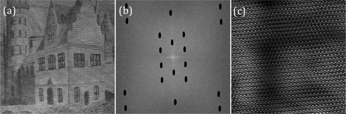
Figure 12 Image of a painting (a), its filtered Fourier transform (b) and the rendered image after filtering (c).

That was a lot of work! It was fun though knowing that how Fourier transform is so useful in image processing. My perception of as a mere long equation totally changed after this activity. I enjoyed very much and I’ve done a heck of a work. For that, I want to give myself a score of 10.

Acknowledgement:

I would like to thank Ms. Krizzia Mañago for reviewing my work.

Reference:

[1] M. Soriano, AP 186 Activity 6: Properties and Applications of 2D Fourier Transform. 2016.

Fourier Transform Model of Image Formation

Our next lesson is about Fourier transform wherein we transform some known functions from time to frequency domain. This is an interesting activity because here Fourier transform is applied to do simple image processing.

The first example is a circular aperture. The function fftshift is applied on the aperture to shift the quadrants. Fast Fourier transform algorithm, known as fft, assumes that the center of the object is indexed first. Therefore, there is a need to shift the quadrants such that they satisfies this assumption. Figure 1 shows the images of a circular aperture and its image when its 4 quadrants are shifted.

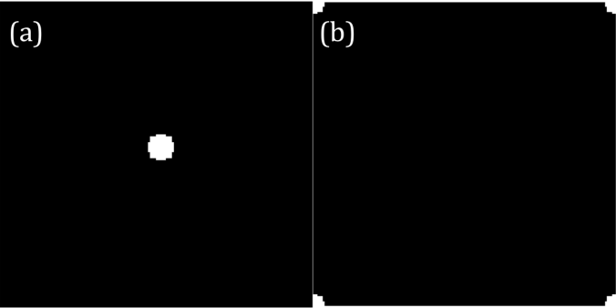
Figure 1. circular aperture (a) and its shifted version (b)

As I mentioned before, Fourier transform brings the image from time to frequency domain. In Fourier space, the values of each pixel are complex. To convince myself, I decomposed the transformed image into real and imaginary parts and I presented them in figure 2.b and 2.c. The pattern obtained when the magnitude of the transformed image is an airy pattern and it is showed in Figure 2.a. Cool! In some classes, we just derive the Fourier transform of some functions but here, we visualize it. I also did this to the Fourier transform of image “A” and the results are in Figure 3.

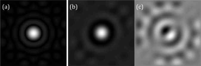
Figure 2. The Fourier transform of circle (a) is composed of real (b) and imaginary parts (c).

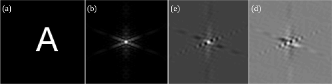
Figure 3. Image of letter “A” (a) and its Fourier transform (b). The transform is further decomposed into its real (e) and imaginary (d) components.

After the circle, I proceeded with corrugated roof, double slit, square function and Gaussian curve. For me, the corrugated roof is the best example to discuss Fourier transform to starters. Fourier transform follows the superposition principle where it is stated that all signals are sums sinusoids with different frequencies and amplitude modulation. A corrugated roof is basically a single sinusoid signal with one constant frequency. Its Fourier transform has 2 peaks equidistant from the origin located on the +/- frequency value as shown in figure 6b. It is a concrete visualization of what the Fourier transform really does to the input signal: it decomposes the input into its frequency components. Another interesting result is the fft of the double slit because it resembles the diffraction pattern of a double slit. This shows that I can also use fft to visualize the diffraction pattern of a given slit. The diffraction pattern of a square aperture also looks the same as its fft which is a sinc function. I displayed the corrugated roof, double slit and square aperture and their Fourier transforms in Figures 4-6.

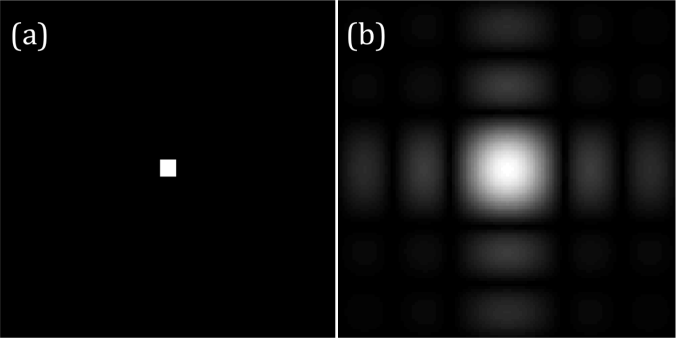
Figure 4. Square aperture (a) and its Fourier transform (b)

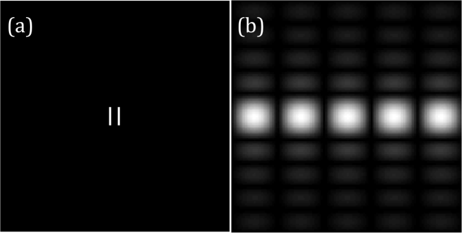
Figure 5. Double slit (a) and its Fourier transform (b)

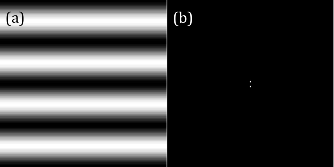
Figure 6. Corrugated roof along x-axis(a) and its Fourier transform (b)

Circular and square aperture, corrugated roof and double slit have some cool fft but the Gaussian aperture is different. The FFT of a Gaussian curve is still a Gaussian curve. Pretty boring isn’t it? But imagine this, if you have Gaussian beam and you propagate it to some distance you will still get a Gaussian beam! Most of the time, laser people wants their laser beam to have a same profile after propagating it at some distance. The Gaussian aperture and its Fourier transform is given in figure 7.

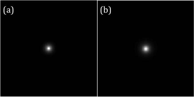
Figure 7. Gaussian aperture (a) and its Fourier transform (b)

 

The next basic concept is convolution. It is a systematic process of combining two signals. Convolution simulates the effects of the imaging systems to the final image registered in the camera sensor. For this section, I used an image of the word “VIP” and it is shown in figure 8d. Due to the finite diameter of the lens, only part of the information of the object is attainable for every imaging system. This is where convolution will come in. I convolved circular apertures with different radii to the 2D Fourier transform of the image to simulate the effect of the finite radius of the lens. The results are presented in figures 8d-e. As the size of the circular aperture becomes smaller, lesser frequencies are brought back to the time domain by inverse Fourier transform therefore the image becomes more and more blurred.

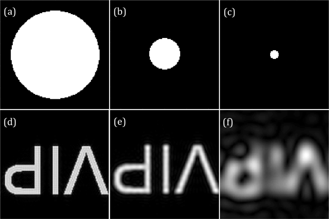
Figure 8. Imaging with different aperture size. Aperture in (a) yields the most slear ‘VIP’ image. The quality of the image degrades as the aperture becomes smaller.

Another image processing technique is the use of correlation to template matching. Here, I use an sentence and letter “A” rendered as images. The goal is to find where the A’s are in the sentence. Both of the images are transformed to Fourier space. The conjugate of the transformed image of the sentence is multiplied to the transformed image of “A”. The result is presented in Figure 9 and it shows that the intensity on the position of A’s in the sentence is higher compared to the rest of the letters.

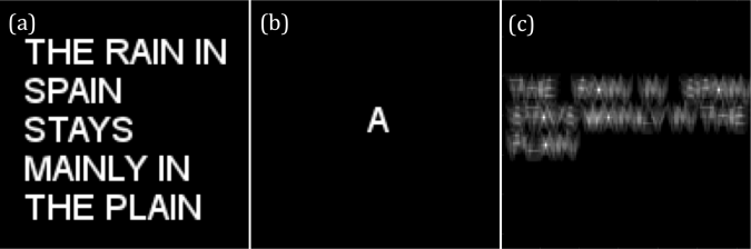
Figure 9. The given pattern (a) is convolved with a template (b) to find the location of the template along the pattern. The bright peaks in (c) pinpoint the location of the template.

For the last part, Convolution is used for edge detection. Using the same “VIP” image and 3×3 matrices with total sum of 0, the vertical and horizontal edges are erased as shown in figure 10. The 3×3 matrices are, a = [-1 -1 -1; 2 2 2;-1 -1 -1], b = [-1 2 -1; -1 2 -1;-1 2 -1], and c = [-1 -1 -1; -1 8 -1; -1 -1 -1] . The edge detected by convolving the “VIP” image to either of the zero sum matrices given is perpendicular to the orientation of the arrays of -1’s from the matrix. The matrix a, for example, detects vertical edges.

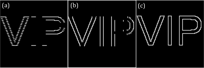
Figure 10. Edge detection using different 3×3 zero sum matrix.

Although this is an introductory activity, it took me a lot of time before I finished it. It is because I want to savor this topic. I would rate myself as 10.

Acknowledgement:

I would like to thank Ms. Krizzia Mañago for reviewing my work.

Reference:

[1] M. Soriano, AP 186 A5 – Fourier Transformation Model of Image Formation. 2016

[2] Smith, Ph.D. By Steven W. “The Scientist and Engineer’s Guide ToDigital Signal ProcessingBy Steven W. Smith, Ph.D.” Convolution. N.p., n.d. Web. 12Oct. 2016. http://www.dspguide.com/ch6.htm

Length and Area Estimation in Images

Our activity last time was about the basics of Scilab. We are now tasked to use it to process an image and measure its area. This, for me, is our first image processing activity. This particular module is about measuring the actual area of a building or any place by their photos.

For this activity, we use Green’s theorem which states that the area inside a curve is equal to the contour integral around it. The area A inside a curve in discrete form is derived and given by:

                                                                            (1)

where x_i and y_i are the pixel coordinates of a point, and x_(i+1) and y_(i+1) are the coordinates of the next point. The equation is the contour integral along the curve necessitating the points to be arranged first in increasing order based on their subtended angles before evaluating the integral.

Unfortunately, I can’t use my Scilab right now right now for some reason that it stopped reading my images. For this activity, I use Matlab instead. Matlab and Scilab are practically the same. Both of them have a built-in function that detects the edges of the shapes in the image and then gives off their corresponding indices. The function is called as edge and you can set the mode for finding the edges. In my case, I use ‘prewitt’ mode. My sample image is a rectangle that has a white fill in it. It is drawn through Microsoft Paint. The imread and rgb2gary function of Matlab is used to load the image and to convert it into grayscale image. The edges of the rectangle are detected using the edge function. The result is a matrix with values-1 and 0- as elements. The indices of the 1’s mark the edges of the input shape. The input image and the result of edge detection are presented in figure 1.

Figure 1. The edge function of Matlab detects the edges of a rectangle (a) and gives off the indices of the edge points. The edge points trace the edges of the shape as shown in (b).

The coordinates of the centroid of the image are subtracted from the coordinates of each edge point. Then, each edge point is ranked in increasing order based on its swept angle. This angle is calculated by getting the inverse tangent of the x and y coordinate of an edge point. The area is calculated using   equation 1.

Using the algorithm in figure 2 the area of the rectangle is 52808 pixel^2 which is approximately the same as the theoretical area of 52812 pixel^2.

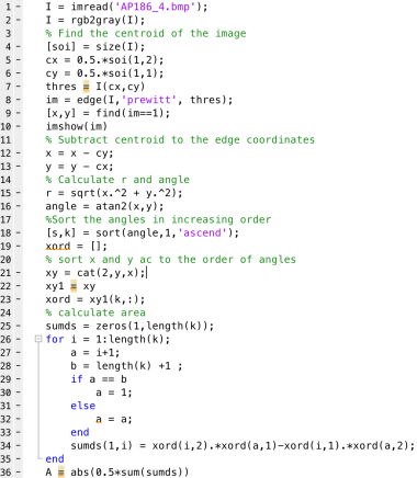Figure 2. Source code from area measurement

The same algorithm is used to calculate the area covered by the College of Science Amphitheater. The image is taken from Google maps. The area of interest is filled with white color and the latter parts are painted with black. The absolute scale of Google maps is used to calculate the scale factor that converts pixel area to real area. Calculated area using Matlab is 4618.1 m^2 which is slightly greater than the actual area by 0.175 % (4610 m^2). The actual area of the College of Science Amphitheater and its edges are shown in figure 3.

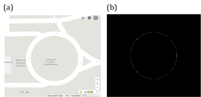Figure 3. Map of CS Amphitheater (a) and its edge (b).

Area measurement is also possible by uploading and analyzing the image of a map or objects in a software named ImageJ. ImageJ is a free image processing software created by National Institutes of Health in US. One can easily use this as the software that can measure the area of interest in the image drawn with a closed curve. By just setting the right scale factor between the pixel distance and actual length between two points inside, ImageJ can calculate the actual area of the object or place.

To demonstrate the process of area measurement tool of ImageJ, the area covered by an ID picture is estimated. The scale factor is set to 156.513 pixels/cm which is done by getting pixel count of a   line drawn between two adjacent centimeter ticks along the measuring tape in the image. The estimated area by ImageJ is 8.688 cm^2. It deviates from the real area, which is 8.670, by 2.08 %. The object of interest is shown in figure 4.

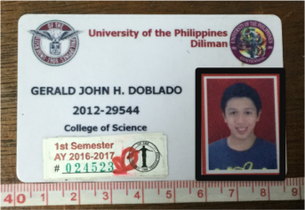Figure 4. The area covered by the ID picture (outlined by the black rectangle) is measured using the analyze tool of ImageJ.

My results are very close to the theoretical areas of the objects I have analyzed. My largest percent error is 2.08%. Therefore, I have done well in this activity. For that, I rate myself as 9.

Acknowledgement:

I would like to thank Ms. Krizzia Mañago for reviewing my work.

Reference:

[1] M. Soriano, Applied Physics 186 A4- Length and Area Estimation in Images. 2014.

Scilab basics

Scilab, like Matlab, is a coding platform that caters efficient matrix handling. The good thing about it is the fact that it is free! Its basic operations are very straightforward – matrix addition and multiplication are as simple as A + B and A*B. Useful for image processing, its procedures are mostly matrix manipulation.

Digital masking is an important tool in learning the basics of image processing and optical simulations. This is done by an element-by-element multiplication of the image and the mask.

For this activity, we are asked to generate 7 different synthetic images: square, sinusoid and grating along x direction, annulus, circular aperture with gaussian transparency, ellipse and cross. Each of them is generated by different functions which I will discuss in detail on the following sections.

The algorithm is basically divided into 3 parts: generation of a 2D grid, implementation of the generating function of the desired synthetic image and visualization of the image. Consider the algorithm for generating a square aperture provided in Figure 1. Line 1 closes all current Scilab figures. Since Scilab does not automatically close all the figures when executing another script, this line does the cleaning job. Lines 2-6 create an nx by ny 2D grid. Lines 7-12 are the implementation parts where the square image is generated. Note that I used A.*A1 in lines 14 and 17 to produce a square. A square is therefore basically done by an element-by-element multiplication of two orthogonal bars with the same thickness. The visualization of this process is given in figure. 2.a-2.c. The surface profile of the square is given in figure 2.d.

 

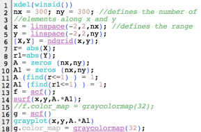Figure 1. Code snippet for square aperture.

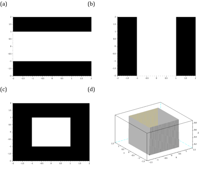
Figure 2. The element-by-element multiplication of (a) and (b) results to a square aperture (c). The profile of this aperture is given in (d).

The next synthetic image is a sinusoid. I generated it by taking the sine of the Y grid. The function is given by:

                                                                  r=sin⁡(nπY)                                      (1)

The equation above replaces the generating function of square aperture. The variable n of equation 1 dictates the number of cycles in the sinusoid image. Note that the Y grid is used because the sinusoid must be along the X direction. The code and generated image are given in figures 3 and 4.

 

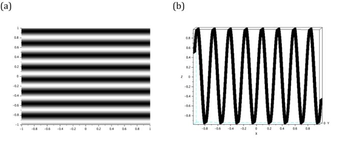Figure 4. The siusoidal image is generated by taking the sine of Y grid. Its line scan is also given to visualize the profile of the image.

 

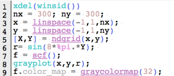Figure 3. Code snippet for sinusoid image.

The binarization of the sinusoid image results to a grating. Using the same code given in figure 3, together with the binarization process, the achieved grating is presented in figure 5.

 

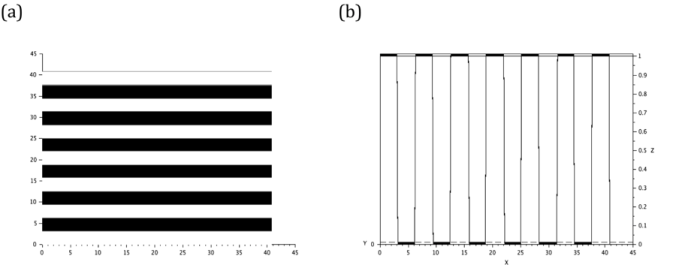Figure 5. The binarization of the sinusoid in previous selections yields a grating (a). The profile (b) of the image is also given.

 

Annulus and circular masks are generated by the same function which is the equation of circle itself r= sqrt(X.^2 + Y.^2). However, the annulus is supposed to be hollow in the inside so I added a condition A (find(r<0.4)) = 0 wherein I punctured a a circle inside the bigger circle. The inner radius of the annulus is equal to the radius of the punctured area. The code snippet and the annulus mask are presented in figures 6 and 7.

 

 

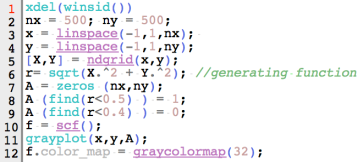Figure 6. Code snippet for annulus.

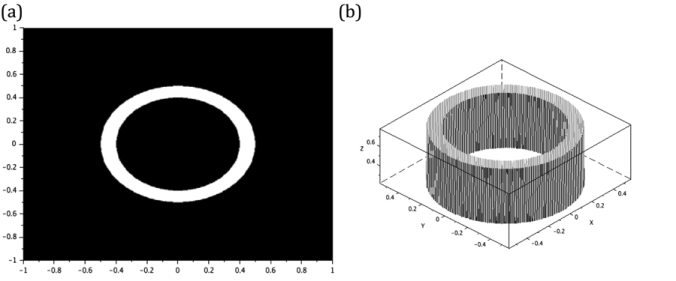Figure 7. The annulus (a) generated has an outer and inner radii of 0.5 and 0.4 respectively. It profile is given in (b).

 

For the image of the ellipse, the function in equation 2 is implemented. First, set the right hand side of the equation 2 to an arbitrary variable r. Then, set all the points enclosed by the curve r into 1. These processes are shown in lines 6 and 9 from the algorithm in figure 8. The lengths of major and minor axes of the ellipse are designated to variables Ma and ma, respectively. The obtained elliptical synthetic image and its surface profile are presented in figure 9.

             X^2/a^2 +Y^2/b^2 =1                 (2)

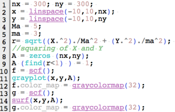Figure 8. Code snippet for ellipse image.

 

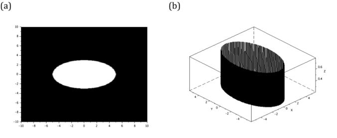Figure 9. The generated ellipse (a), with major and minor axis lengths of 5 and 3 units respectively, and its profile (b) are shown here.

 

The next image is a cross. I visualize it as a superposition of two orthogonal rectangles. The generation of a rectangular aperture is similar to the process of creating a square aperture but the side lengths are not equal for this case. Lines 11-18 of figure 10 create two perpendicular rectangles. Line 19, on the other hand, superimposes the rectangles. Therefore, this shows that I can use matrix addition and element-by-element multiplication simultaneously to create my desired image. However, adding the two rectangles means that the intersection of their areas has more irradiance compared to the lateral parts of the cross. Using the lines 19-27, I smoothen the profile of the cross image by equating all the gray values inside the image to 1. The image and profile of the cross are both given in figure 11.

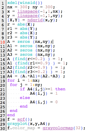Figure 10. Code snippet for cross

 

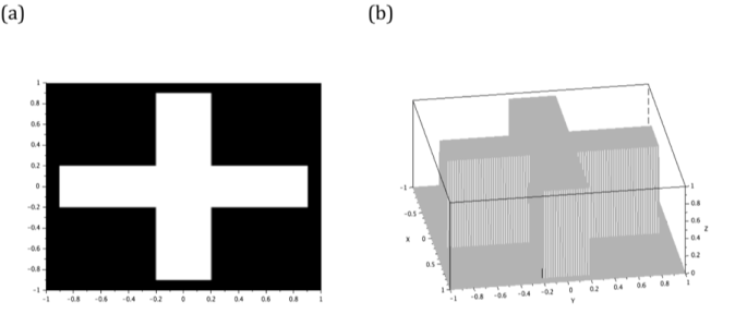Figure 11. The cross (a) is generated by adding two orthogonal 1.8 x 0.4rectangles. Its profile is also given here (b).

 

The final image is a gaussian mask. It is known to blur the image impinged to it. [3] Its equation is given by:

                                               G(x)= a*exp((-(x-b)^2)/(2c^2 ))               (3)

where a is the peak value, b is the location of the center and c is the standard deviation. It is used as the generating function of the image.

The irradiance of gaussian mask image is concentrated inside the standard deviation (c). Hence, when another image is masked by a gaussian mask, the center detail remains clear as long as it is inside the radius equal to c. The remaining parts of the image inside this radius are blurred. The gaussian mask and its profile are presented in figure 13.

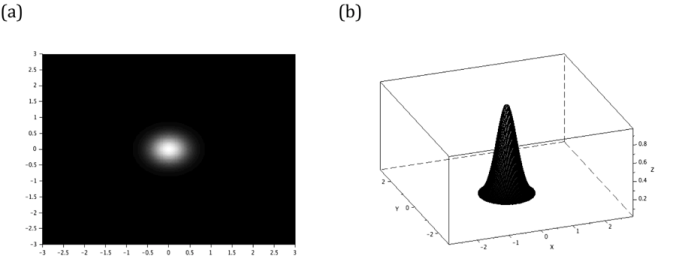Figure 13. The gaussian mask (a) and its profile (b).

 

To sum up, I generated all the 7 images using some matrix manipulations available in Scilab. Hence, I give myself a score of 8. I think that some of my codes are lengthy even though I only performed all the steps that Dr. Soriano asked me to do.

Personally, I enjoy this activity because this teaches me how to make different apertures to play with light.

 

Acknowledgement:

I would like to thank Ms. Krizzia Mañago for reviewing my work and Ms. Niña Zambale for sharing her way of discussing this activity.

References:

[1] http://www.scilab.org/

[2] M. Soriano, Applied Physics 186 A3 – Scilab Basics. 2016

[3] http://homepages.inf.ed.ac.uk/rbf/HIPR2/gsmooth.htm

 

Digital Scanning

The goal of this activity is to reconstruct any printed graph by relating the pixel coordinates of its data points to their actual x and y values.   A graph from a journal is scanned using a flatbed scanner. [1] The image is viewed and edited in GIMP software. The scanned image is slightly rotated to make it upright such that the x and y axes of the plot are parallel horizontally and vertically with the image itself. The scanned and rotated image is shown in figure 1.

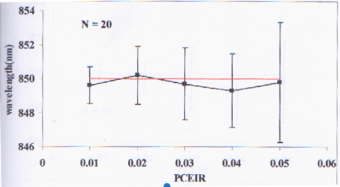
Figure 1. The scanned plot. This activity aims to get the approximate x and y values of each point on the graph.

 

The first task is to count the number of pixels present between two consecutive ticks along an axis from which I started with the x-axis. By placing the cursor on one point of the plot, the position of the pixel coordinates (located at the bottom left of the GIMP window) is obtained. The number of pixels across two consecutive ticks is recorded in a spreadsheet. Note that in the first part, the axes of the image are assured to be horizontally (x) and vertically (y) parallel with the image itself. Therefore, in this case, only the x pixel coordinate is the one that is changing. The y pixel coordinate remained constant as the pointer jumped from one tick to the next. The array of pixel counts for the x axis is tabulated and averaged. Then, the increment value between two consecutive ticks is divided by the calculated average. The obtained ratio could then relate the x pixel position of a point and its real x value. This process is also done for the y axis of the plot but this time, the x pixel coordinate remained constant. Like the case of the x-axis, the obtained ratio for the y-axis relates the y pixel position of a point and its real y value. I summarized the numerical values in table 1.

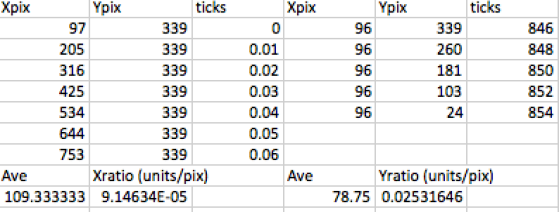
Table 1. The pixel coordinates of the ticks for each axis was recorded. Using Xpix and Ypix values, the ratios that convert image pixel coordinates to real x and y values were derived.

 

The conversion equations from pixel coordinates to the real coordinates are given by:

X = Xratio*(Xpix-97)

Y = Yratio*(Ypix-339)

The second and final task is to use the conversion ratios of x and y pixel coordinates to reconstruct the graph. The pixel coordinates of 5 data points from figure 1 are listed in a spreadsheet. Since the origins of the scanned plot and pixel coordinates are not at the same place, the x and y pixel coordinates of the original origin are subtracted from the data sets to offset the translation of one coordinate system with respect to the other. Finally, the x and y pixel values of each point are multiplied to the x and y conversion ratios. I therefore recovered the original x and y values of the data points. The reconstructed x and y values of the points are listed in table 2.

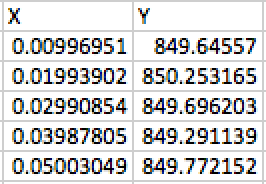
Table 2. Reconstructed data points. I derived the real x and y values of the data points based on their pixel coordinates.

I superimposed the scanned image and my plot in figure 2 and it turned out that they are very similar. Thus, I successfully reconstructed the original plot by carefully implementing the steps given by my instructor. For this activity, I rate myself as 9 since my plot resembles the original one.

Figure 2. Superimposed image and reconstructed plot.

 

Acknowledgement

I would like to thank Ms. Krizzia Mañago for reviewing my work.

References:

[1] J.E. Tio. Simulation of a One Dimensional Photonic Crystal with Defects. October 2001.

[2] M. Soriano, Applied Physics 186 A2 – Digital Scanning. 2016.