Length and Area Estimation in Images

Our activity last time was about the basics of Scilab. We are now tasked to use it to process an image and measure its area. This, for me, is our first image processing activity. This particular module is about measuring the actual area of a building or any place by their photos.

For this activity, we use Green’s theorem which states that the area inside a curve is equal to the contour integral around it. The area A inside a curve in discrete form is derived and given by:

                                                                            (1)

where x_i and y_i are the pixel coordinates of a point, and x_(i+1) and y_(i+1) are the coordinates of the next point. The equation is the contour integral along the curve necessitating the points to be arranged first in increasing order based on their subtended angles before evaluating the integral.

Unfortunately, I can’t use my Scilab right now right now for some reason that it stopped reading my images. For this activity, I use Matlab instead. Matlab and Scilab are practically the same. Both of them have a built-in function that detects the edges of the shapes in the image and then gives off their corresponding indices. The function is called as edge and you can set the mode for finding the edges. In my case, I use ‘prewitt’ mode. My sample image is a rectangle that has a white fill in it. It is drawn through Microsoft Paint. The imread and rgb2gary function of Matlab is used to load the image and to convert it into grayscale image. The edges of the rectangle are detected using the edge function. The result is a matrix with values-1 and 0- as elements. The indices of the 1’s mark the edges of the input shape. The input image and the result of edge detection are presented in figure 1.

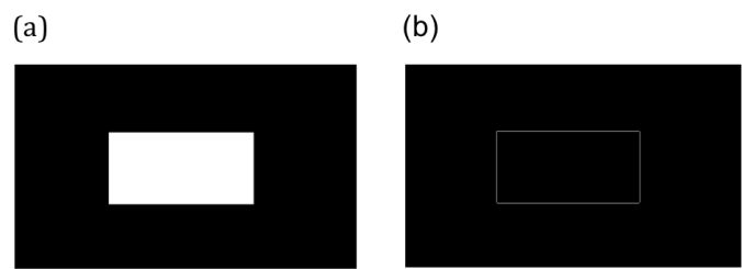
Figure 1. The edge function of Matlab detects the edges of a rectangle (a) and gives off the indices of the edge points. The edge points trace the edges of the shape as shown in (b).

The coordinates of the centroid of the image are subtracted from the coordinates of each edge point. Then, each edge point is ranked in increasing order based on its swept angle. This angle is calculated by getting the inverse tangent of the x and y coordinate of an edge point. The area is calculated using   equation 1.

Using the algorithm in figure 2 the area of the rectangle is 52808 pixel^2 which is approximately the same as the theoretical area of 52812 pixel^2.

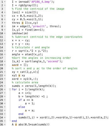
Figure 2. Source code from area measurement

The same algorithm is used to calculate the area covered by the College of Science Amphitheater. The image is taken from Google maps. The area of interest is filled with white color and the latter parts are painted with black. The absolute scale of Google maps is used to calculate the scale factor that converts pixel area to real area. Calculated area using Matlab is 4618.1 m^2 which is slightly greater than the actual area by 0.175 % (4610 m^2). The actual area of the College of Science Amphitheater and its edges are shown in figure 3.

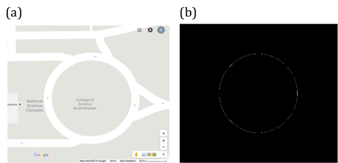
Figure 3. Map of CS Amphitheater (a) and its edge (b).

Area measurement is also possible by uploading and analyzing the image of a map or objects in a software named ImageJ. ImageJ is a free image processing software created by National Institutes of Health in US. One can easily use this as the software that can measure the area of interest in the image drawn with a closed curve. By just setting the right scale factor between the pixel distance and actual length between two points inside, ImageJ can calculate the actual area of the object or place.

To demonstrate the process of area measurement tool of ImageJ, the area covered by an ID picture is estimated. The scale factor is set to 156.513 pixels/cm which is done by getting pixel count of a   line drawn between two adjacent centimeter ticks along the measuring tape in the image. The estimated area by ImageJ is 8.688 cm^2. It deviates from the real area, which is 8.670, by 2.08 %. The object of interest is shown in figure 4.

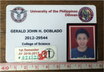
Figure 4. The area covered by the ID picture (outlined by the black rectangle) is measured using the analyze tool of ImageJ.

My results are very close to the theoretical areas of the objects I have analyzed. My largest percent error is 2.08%. Therefore, I have done well in this activity. For that, I rate myself as 9.

Acknowledgement:

I would like to thank Ms. Krizzia Mañago for reviewing my work.

Reference:

[1] M. Soriano, Applied Physics 186 A4- Length and Area Estimation in Images. 2014.

Scilab basics

Scilab, like Matlab, is a coding platform that caters efficient matrix handling. The good thing about it is the fact that it is free! Its basic operations are very straightforward – matrix addition and multiplication are as simple as A + B and A*B. Useful for image processing, its procedures are mostly matrix manipulation.

Digital masking is an important tool in learning the basics of image processing and optical simulations. This is done by an element-by-element multiplication of the image and the mask.

For this activity, we are asked to generate 7 different synthetic images: square, sinusoid and grating along x direction, annulus, circular aperture with gaussian transparency, ellipse and cross. Each of them is generated by different functions which I will discuss in detail on the following sections.

The algorithm is basically divided into 3 parts: generation of a 2D grid, implementation of the generating function of the desired synthetic image and visualization of the image. Consider the algorithm for generating a square aperture provided in Figure 1. Line 1 closes all current Scilab figures. Since Scilab does not automatically close all the figures when executing another script, this line does the cleaning job. Lines 2-6 create an nx by ny 2D grid. Lines 7-12 are the implementation parts where the square image is generated. Note that I used A.*A1 in lines 14 and 17 to produce a square. A square is therefore basically done by an element-by-element multiplication of two orthogonal bars with the same thickness. The visualization of this process is given in figure. 2.a-2.c. The surface profile of the square is given in figure 2.d.

 

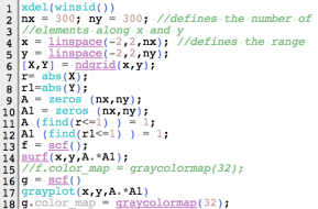
Figure 1. Code snippet for square aperture.

Figure 2. The element-by-element multiplication of (a) and (b) results to a square aperture (c). The profile of this aperture is given in (d).

The next synthetic image is a sinusoid. I generated it by taking the sine of the Y grid. The function is given by:

                                                                  r=sin⁡(nπY)                                      (1)

The equation above replaces the generating function of square aperture. The variable n of equation 1 dictates the number of cycles in the sinusoid image. Note that the Y grid is used because the sinusoid must be along the X direction. The code and generated image are given in figures 3 and 4.

 

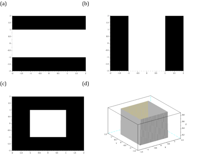
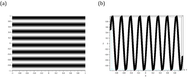
Figure 4. The siusoidal image is generated by taking the sine of Y grid. Its line scan is also given to visualize the profile of the image.

 

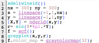
Figure 3. Code snippet for sinusoid image.

The binarization of the sinusoid image results to a grating. Using the same code given in figure 3, together with the binarization process, the achieved grating is presented in figure 5.

 

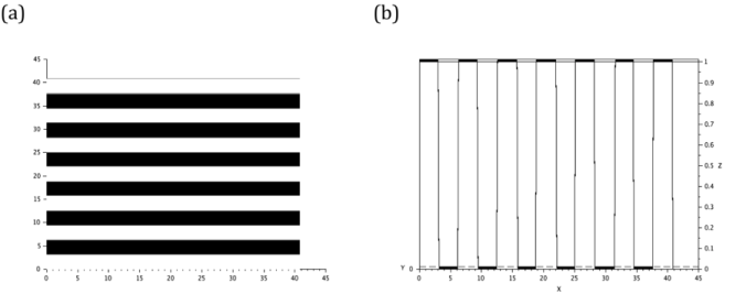
Figure 5. The binarization of the sinusoid in previous selections yields a grating (a). The profile (b) of the image is also given.

 

Annulus and circular masks are generated by the same function which is the equation of circle itself r= sqrt(X.^2 + Y.^2). However, the annulus is supposed to be hollow in the inside so I added a condition A (find(r<0.4)) = 0 wherein I punctured a a circle inside the bigger circle. The inner radius of the annulus is equal to the radius of the punctured area. The code snippet and the annulus mask are presented in figures 6 and 7.

 

 

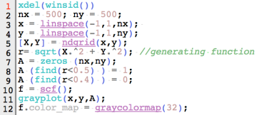
Figure 6. Code snippet for annulus.

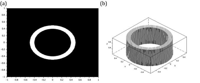
Figure 7. The annulus (a) generated has an outer and inner radii of 0.5 and 0.4 respectively. It profile is given in (b).

 

For the image of the ellipse, the function in equation 2 is implemented. First, set the right hand side of the equation 2 to an arbitrary variable r. Then, set all the points enclosed by the curve r into 1. These processes are shown in lines 6 and 9 from the algorithm in figure 8. The lengths of major and minor axes of the ellipse are designated to variables Ma and ma, respectively. The obtained elliptical synthetic image and its surface profile are presented in figure 9.

             X^2/a^2 +Y^2/b^2 =1                 (2)

Figure 8. Code snippet for ellipse image.

 

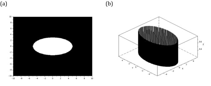
Figure 9. The generated ellipse (a), with major and minor axis lengths of 5 and 3 units respectively, and its profile (b) are shown here.

 

The next image is a cross. I visualize it as a superposition of two orthogonal rectangles. The generation of a rectangular aperture is similar to the process of creating a square aperture but the side lengths are not equal for this case. Lines 11-18 of figure 10 create two perpendicular rectangles. Line 19, on the other hand, superimposes the rectangles. Therefore, this shows that I can use matrix addition and element-by-element multiplication simultaneously to create my desired image. However, adding the two rectangles means that the intersection of their areas has more irradiance compared to the lateral parts of the cross. Using the lines 19-27, I smoothen the profile of the cross image by equating all the gray values inside the image to 1. The image and profile of the cross are both given in figure 11.

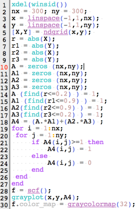
Figure 10. Code snippet for cross

 

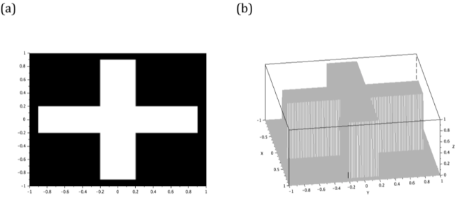
Figure 11. The cross (a) is generated by adding two orthogonal 1.8 x 0.4rectangles. Its profile is also given here (b).

 

The final image is a gaussian mask. It is known to blur the image impinged to it. [3] Its equation is given by:

                                               G(x)= a*exp((-(x-b)^2)/(2c^2 ))               (3)

where a is the peak value, b is the location of the center and c is the standard deviation. It is used as the generating function of the image.

The irradiance of gaussian mask image is concentrated inside the standard deviation (c). Hence, when another image is masked by a gaussian mask, the center detail remains clear as long as it is inside the radius equal to c. The remaining parts of the image inside this radius are blurred. The gaussian mask and its profile are presented in figure 13.

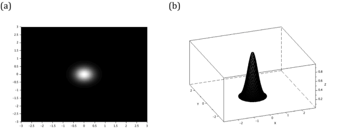
Figure 13. The gaussian mask (a) and its profile (b).

 

To sum up, I generated all the 7 images using some matrix manipulations available in Scilab. Hence, I give myself a score of 8. I think that some of my codes are lengthy even though I only performed all the steps that Dr. Soriano asked me to do.

Personally, I enjoy this activity because this teaches me how to make different apertures to play with light.

 

Acknowledgement:

I would like to thank Ms. Krizzia Mañago for reviewing my work and Ms. Niña Zambale for sharing her way of discussing this activity.

References:

[1] http://www.scilab.org/

[2] M. Soriano, Applied Physics 186 A3 – Scilab Basics. 2016

[3] http://homepages.inf.ed.ac.uk/rbf/HIPR2/gsmooth.htm

 

Digital Scanning

The goal of this activity is to reconstruct any printed graph by relating the pixel coordinates of its data points to their actual x and y values.   A graph from a journal is scanned using a flatbed scanner. [1] The image is viewed and edited in GIMP software. The scanned image is slightly rotated to make it upright such that the x and y axes of the plot are parallel horizontally and vertically with the image itself. The scanned and rotated image is shown in figure 1.

Figure 1. The scanned plot. This activity aims to get the approximate x and y values of each point on the graph.

 

The first task is to count the number of pixels present between two consecutive ticks along an axis from which I started with the x-axis. By placing the cursor on one point of the plot, the position of the pixel coordinates (located at the bottom left of the GIMP window) is obtained. The number of pixels across two consecutive ticks is recorded in a spreadsheet. Note that in the first part, the axes of the image are assured to be horizontally (x) and vertically (y) parallel with the image itself. Therefore, in this case, only the x pixel coordinate is the one that is changing. The y pixel coordinate remained constant as the pointer jumped from one tick to the next. The array of pixel counts for the x axis is tabulated and averaged. Then, the increment value between two consecutive ticks is divided by the calculated average. The obtained ratio could then relate the x pixel position of a point and its real x value. This process is also done for the y axis of the plot but this time, the x pixel coordinate remained constant. Like the case of the x-axis, the obtained ratio for the y-axis relates the y pixel position of a point and its real y value. I summarized the numerical values in table 1.

Table 1. The pixel coordinates of the ticks for each axis was recorded. Using Xpix and Ypix values, the ratios that convert image pixel coordinates to real x and y values were derived.

 

The conversion equations from pixel coordinates to the real coordinates are given by:

X = Xratio*(Xpix-97)

Y = Yratio*(Ypix-339)

The second and final task is to use the conversion ratios of x and y pixel coordinates to reconstruct the graph. The pixel coordinates of 5 data points from figure 1 are listed in a spreadsheet. Since the origins of the scanned plot and pixel coordinates are not at the same place, the x and y pixel coordinates of the original origin are subtracted from the data sets to offset the translation of one coordinate system with respect to the other. Finally, the x and y pixel values of each point are multiplied to the x and y conversion ratios. I therefore recovered the original x and y values of the data points. The reconstructed x and y values of the points are listed in table 2.

Table 2. Reconstructed data points. I derived the real x and y values of the data points based on their pixel coordinates.

I superimposed the scanned image and my plot in figure 2 and it turned out that they are very similar. Thus, I successfully reconstructed the original plot by carefully implementing the steps given by my instructor. For this activity, I rate myself as 9 since my plot resembles the original one.

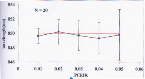
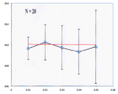
Figure 2. Superimposed image and reconstructed plot.

 

Acknowledgement

I would like to thank Ms. Krizzia Mañago for reviewing my work.

References:

[1] J.E. Tio. Simulation of a One Dimensional Photonic Crystal with Defects. October 2001.

[2] M. Soriano, Applied Physics 186 A2 – Digital Scanning. 2016.