Properties and Applications of 2D Fourier Transform

This activity is about numerical signal filtering in Fourier space. The the goal is to work on the Fourier transform of some images, filter out the unnecessary frequency signals and then render it. Before that, we explore first two properties of 2D Fourier transform: anamorphism and rotation property.

First, I want to talk about anamorphism. The dimension of Fourier space is the inverse of the dimension of the image. This tells that what is large in image space will be small in Fourier space. This property is called anamorphism. Consider now the tall rectangle in (a) of figure 1. It has wider extent along the vertical (y) axis compared to its counterpart in horizontal (x) axis. Therefore, its Fourier transform, which is a sinc function, is wider along the x-axis compared to the y-axis as shown in figure 1b. However, when the wide rectangle is transformed, the result is a sinc function that is wider along the y-axis.

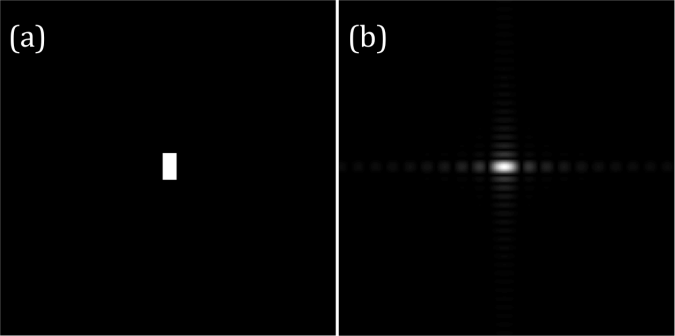
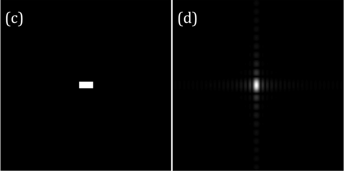
Figure 1. Tall (a) and wide (c) rectangles and their Fourier transforms (b) and (d) respectively.

To demonstrate anamorphism to other patterns, let’s have a look on the Fourier transforms of two dots with different spacing in figures 2. The Fourier transform for this case is composed of vertical bars. It is clearly seen that the as the dots become farther away from each other, the spacing of the bars in Fourier space also increases.

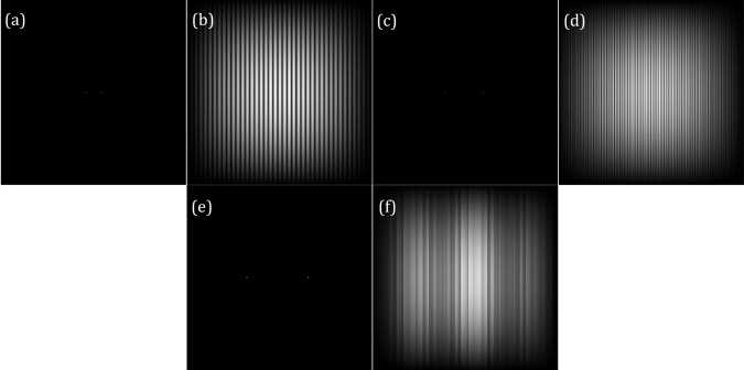
       Figure 2 The set of two dots in (a), (c) and (e) with different separation distances and their Fourier transforms in (b), (d), and (f) respectively.

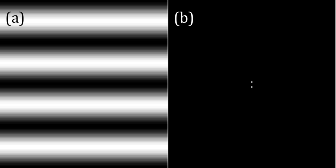
            For the rotation property of Fourier transform, consider now a rotated sinusoid or corrugated roof about the origin. The sinusoid is z = sin(2πfy) with frequency is f = 4 Hz and its Fourier transform is composed of two Dirac deltas located on its frequency as shown in figures 3a and 3b. I also increased the frequency to 20 Hz and 30 Hz. As expected, the Dirac deltas become farther and farther apart as the frequency is increased (refer to figures 3c-e). Images has no negative values therefore to simulate a sinusoid captured by a camera, a constant bias (also known as DC signal) must be added to it. This added value has no frequency so The Fourier transform of the simulated image has a large peak on f = 0. This DC signal obscures the sinusoid signal for it has larger magnitude which is why only the central peek is visible in figure 3g. Therefore, to recover the true signal, this DC signal should be removed in Fourier space. The bias can also be a non-constant function such as another sinusoid. If this bias is added the original signal, the result is in figure 6.Its Fourier transform, However, it has 4 peaks (refer to figure 6b) pinpointing the frequencies of the original signal and the bias. To recover the original signal, the frequency of the bias must be removed in Fourier space before rendering back to the original space of the image.

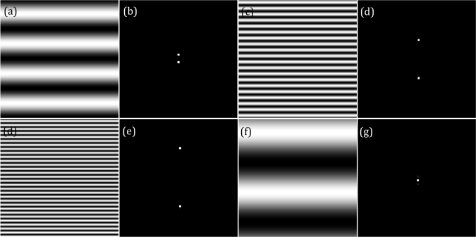
Figure 3 Sinusoids with f = 4 Hz (a), 20 Hz (c) and 30 Hz (d) and their Fourier transforms (b), (d) and (e). The biased sinusoid and its Fourier transform are given , ,however, in (f) and (g).

Moving on, I rotated the sinusiod by modifying its phase term such that new function is z = sin(2πf(ysin(θ) + xcos(θ))) where θ is the rotation angle with respect to the x-axis. The sinusoid is rotated by θ = 45, 90, and 135 degrees. As a result, the Dirac deltas in Fourier space rotates as well in the same direction of θ. The rotated sinusoids and their Fourier transforms were given in figure 4.

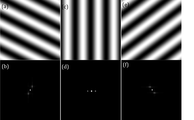
Figure 4 Rotated sinusoids-(a), (c) and (e)- and their Fourier transforms in (b), (d) and (f).

We now investigate the transform a sinusoid multiplied with another sinusoid. Their frequencies are 4 Hz and 8 Hz respectively and the new function is u0 = sin(2π4y).*sin(2π8x). The results were presented in figure 5. The 4 off-centered peaks in Fourier space are located in points (4,8), (-4,8), (4,-8) ,and (-4,-8). Therefore, the multiplied sinusoid modulated such that their frequencies pair up forming a new set.

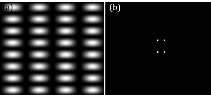
Figure 5 Product of two sinusoids (a) and their Fourier transform (b).

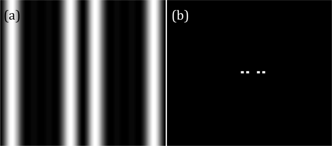
Figure 6 Sum of two sinusoids (a) and their Fourier transform (b).

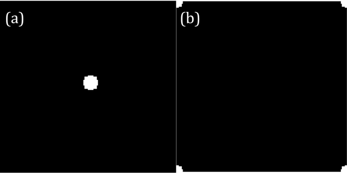
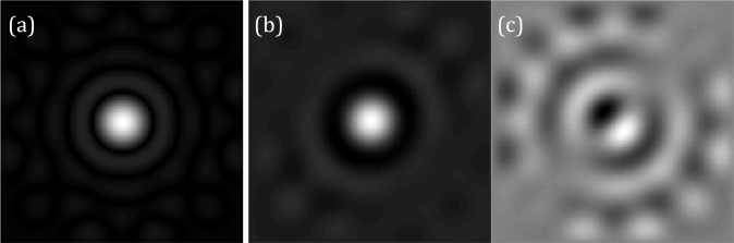
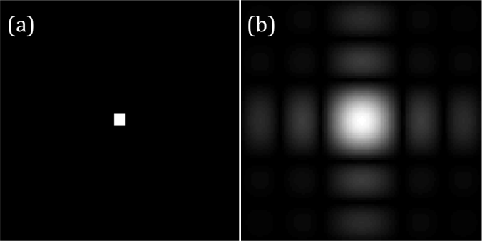
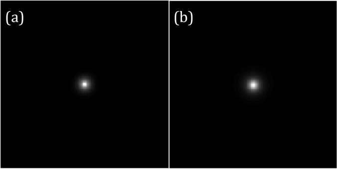
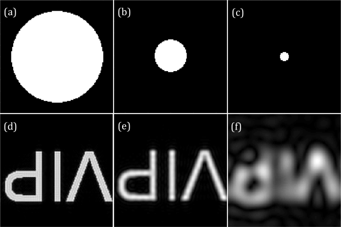
Before we proceed to the image processing techniques, let’s observe first Dirac delta function and its Fourier transform. Dirac delta function is simulated by assigning one pixel to be one and the rest have 0 value. When to two Dirac deltas equidistant about the origin and placed along the x-axis are transformed in Fourier space, the result is composed of equally spaced vertical bars. When the Dirac deltas are replaced by rectangular, circular or Gaussian function, their Fourier transforms have undulations inside the envelopes which are the transforms of these objects(i.e. F{square aperture} = sinc function) as shown in figure7. However, as their dimensions become smaller, their Fourier transforms are approximately the same as the Dirac deltas’.


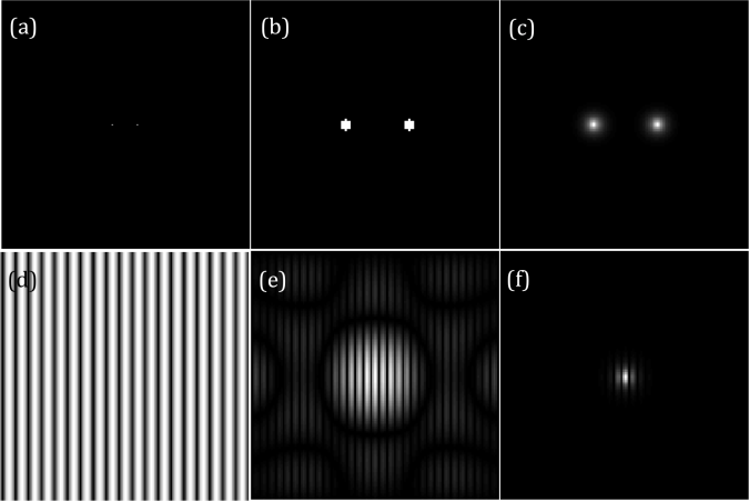
Figure 7 The Fourier transforms of 2 dots (a), 2 circles (b) and 2 gaussian apertures (c) are given in (d), (e) and (f) respectively.

Another exciting fact about Dirac delta is the fact that it brings the function convolved to it on its present location. I used a random 3×3 pattern to demonstrate it. It can be seen in figure 8. that the convolution of the Dirac deltas with the pattern resulted to image with miniature version of the pattern on the location of the Dirac deltas.

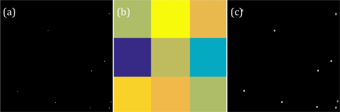
Figure 8. The convolution of Dirac deltas (a) and random pattern(b) results to (c).

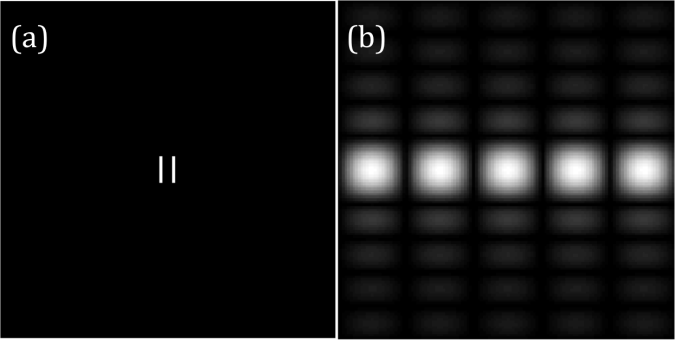
Finally, the Fourier transform of an array of Dirac deltas. The contribution of the Dirac deltas along the y axis modulates the Fourier transforms of Dirac deltas lining up the x axis and forming an array of sinc functions and it is shown in figure 9. The number of bright peaks in Fourier space is equal to the number of Dirac deltas.

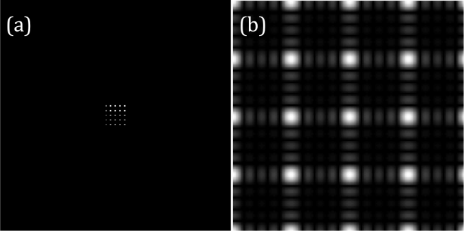
Figure 9. A 5×5 matrix of Dirac Deltas (a) and its Fourier transform (b)

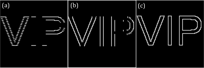
After a long discussion about the properties of Fourier transform, we are ready to do dome image processing using this as a tool. The first image to be processed is from the Lunar Orbiter. It is a panorama with evident bright lines between each stitched frame. We want to eliminate these lines to render a smooth image. Notice that these horizontal lines occur periodically in the image. Therefore, its Fourier transform is composed of points along the y-axis. I filtered it out by blocking the signal along the y-axis of its transform and the result is a smooth picture as shown in figure 10c

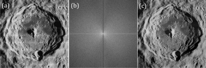
Figure 10. Image from Lunar orbiter (a), its filtered Fourier transform (b) and the rendered image after filtering (c).

The next images is a picture of fingerprint. What we want is to enhance the contrast of the ridges of the patterns. The image has tightly spaced periodic patterns so the Fourier transform of this has more signal on higher frequencies. Also, the periodic lines are oblique so I expect that the frequency signals traces a round path. I filtered out the signals with lower frequencies except the DC term. The ridges become more pronounced than the previous image and it was shown in figure 11.

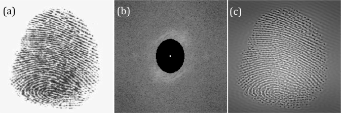
Figure11. Image of fingerprint (a), its filtered Fourier transform (b) and the rendered image after filtering (c).

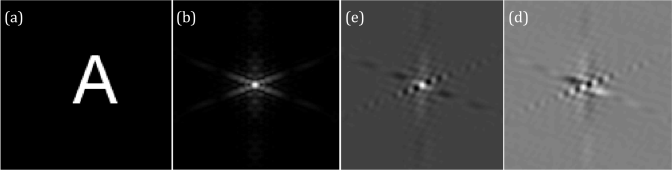
For the last part we were tasked to obtain the canvass weave of a painting. The weave pattern is evident from the painting itself. It is a rotated periodic pattern which seems to be sinusoids that are either superimposed or multiplied to each other. Knowing this, I designed a filter that extracts the peaks corresponding to these sinusoids in Fourier space and projected it back to original plane. The result is an image of just the canvass weave. The original image of painting, its Fourier transform ,and its canvass weave are shown in figure 12

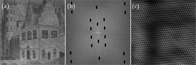
Figure 12 Image of a painting (a), its filtered Fourier transform (b) and the rendered image after filtering (c).

That was a lot of work! It was fun though knowing that how Fourier transform is so useful in image processing. My perception of as a mere long equation totally changed after this activity. I enjoyed very much and I’ve done a heck of a work. For that, I want to give myself a score of 10.

Acknowledgement:

I would like to thank Ms. Krizzia Mañago for reviewing my work.

Reference:

[1] M. Soriano, AP 186 Activity 6: Properties and Applications of 2D Fourier Transform. 2016.

Fourier Transform Model of Image Formation

Our next lesson is about Fourier transform wherein we transform some known functions from time to frequency domain. This is an interesting activity because here Fourier transform is applied to do simple image processing.

The first example is a circular aperture. The function fftshift is applied on the aperture to shift the quadrants. Fast Fourier transform algorithm, known as fft, assumes that the center of the object is indexed first. Therefore, there is a need to shift the quadrants such that they satisfies this assumption. Figure 1 shows the images of a circular aperture and its image when its 4 quadrants are shifted.

Figure 1. circular aperture (a) and its shifted version (b)

As I mentioned before, Fourier transform brings the image from time to frequency domain. In Fourier space, the values of each pixel are complex. To convince myself, I decomposed the transformed image into real and imaginary parts and I presented them in figure 2.b and 2.c. The pattern obtained when the magnitude of the transformed image is an airy pattern and it is showed in Figure 2.a. Cool! In some classes, we just derive the Fourier transform of some functions but here, we visualize it. I also did this to the Fourier transform of image “A” and the results are in Figure 3.

Figure 2. The Fourier transform of circle (a) is composed of real (b) and imaginary parts (c).

Figure 3. Image of letter “A” (a) and its Fourier transform (b). The transform is further decomposed into its real (e) and imaginary (d) components.

After the circle, I proceeded with corrugated roof, double slit, square function and Gaussian curve. For me, the corrugated roof is the best example to discuss Fourier transform to starters. Fourier transform follows the superposition principle where it is stated that all signals are sums sinusoids with different frequencies and amplitude modulation. A corrugated roof is basically a single sinusoid signal with one constant frequency. Its Fourier transform has 2 peaks equidistant from the origin located on the +/- frequency value as shown in figure 6b. It is a concrete visualization of what the Fourier transform really does to the input signal: it decomposes the input into its frequency components. Another interesting result is the fft of the double slit because it resembles the diffraction pattern of a double slit. This shows that I can also use fft to visualize the diffraction pattern of a given slit. The diffraction pattern of a square aperture also looks the same as its fft which is a sinc function. I displayed the corrugated roof, double slit and square aperture and their Fourier transforms in Figures 4-6.

Figure 4. Square aperture (a) and its Fourier transform (b)

Figure 5. Double slit (a) and its Fourier transform (b)

Figure 6. Corrugated roof along x-axis(a) and its Fourier transform (b)

Circular and square aperture, corrugated roof and double slit have some cool fft but the Gaussian aperture is different. The FFT of a Gaussian curve is still a Gaussian curve. Pretty boring isn’t it? But imagine this, if you have Gaussian beam and you propagate it to some distance you will still get a Gaussian beam! Most of the time, laser people wants their laser beam to have a same profile after propagating it at some distance. The Gaussian aperture and its Fourier transform is given in figure 7.

Figure 7. Gaussian aperture (a) and its Fourier transform (b)

 

The next basic concept is convolution. It is a systematic process of combining two signals. Convolution simulates the effects of the imaging systems to the final image registered in the camera sensor. For this section, I used an image of the word “VIP” and it is shown in figure 8d. Due to the finite diameter of the lens, only part of the information of the object is attainable for every imaging system. This is where convolution will come in. I convolved circular apertures with different radii to the 2D Fourier transform of the image to simulate the effect of the finite radius of the lens. The results are presented in figures 8d-e. As the size of the circular aperture becomes smaller, lesser frequencies are brought back to the time domain by inverse Fourier transform therefore the image becomes more and more blurred.

Figure 8. Imaging with different aperture size. Aperture in (a) yields the most slear ‘VIP’ image. The quality of the image degrades as the aperture becomes smaller.

Another image processing technique is the use of correlation to template matching. Here, I use an sentence and letter “A” rendered as images. The goal is to find where the A’s are in the sentence. Both of the images are transformed to Fourier space. The conjugate of the transformed image of the sentence is multiplied to the transformed image of “A”. The result is presented in Figure 9 and it shows that the intensity on the position of A’s in the sentence is higher compared to the rest of the letters.

Figure 9. The given pattern (a) is convolved with a template (b) to find the location of the template along the pattern. The bright peaks in (c) pinpoint the location of the template.

For the last part, Convolution is used for edge detection. Using the same “VIP” image and 3×3 matrices with total sum of 0, the vertical and horizontal edges are erased as shown in figure 10. The 3×3 matrices are, a = [-1 -1 -1; 2 2 2;-1 -1 -1], b = [-1 2 -1; -1 2 -1;-1 2 -1], and c = [-1 -1 -1; -1 8 -1; -1 -1 -1] . The edge detected by convolving the “VIP” image to either of the zero sum matrices given is perpendicular to the orientation of the arrays of -1’s from the matrix. The matrix a, for example, detects vertical edges.

Figure 10. Edge detection using different 3×3 zero sum matrix.

Although this is an introductory activity, it took me a lot of time before I finished it. It is because I want to savor this topic. I would rate myself as 10.

Acknowledgement:

I would like to thank Ms. Krizzia Mañago for reviewing my work.

Reference:

[1] M. Soriano, AP 186 A5 – Fourier Transformation Model of Image Formation. 2016

[2] Smith, Ph.D. By Steven W. “The Scientist and Engineer’s Guide ToDigital Signal ProcessingBy Steven W. Smith, Ph.D.” Convolution. N.p., n.d. Web. 12Oct. 2016. http://www.dspguide.com/ch6.htm