The goal of this activity is to reconstruct any printed graph by relating the pixel coordinates of its data points to their actual x and y values. A graph from a journal is scanned using a flatbed scanner. [1] The image is viewed and edited in GIMP software. The scanned image is slightly rotated to make it upright such that the x and y axes of the plot are parallel horizontally and vertically with the image itself. The scanned and rotated image is shown in figure 1.
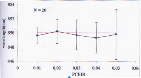
Figure 1. The scanned plot. This activity aims to get the approximate x and y values of each point on the graph.
The first task is to count the number of pixels present between two consecutive ticks along an axis from which I started with the x-axis. By placing the cursor on one point of the plot, the position of the pixel coordinates (located at the bottom left of the GIMP window) is obtained. The number of pixels across two consecutive ticks is recorded in a spreadsheet. Note that in the first part, the axes of the image are assured to be horizontally (x) and vertically (y) parallel with the image itself. Therefore, in this case, only the x pixel coordinate is the one that is changing. The y pixel coordinate remained constant as the pointer jumped from one tick to the next. The array of pixel counts for the x axis is tabulated and averaged. Then, the increment value between two consecutive ticks is divided by the calculated average. The obtained ratio could then relate the x pixel position of a point and its real x value. This process is also done for the y axis of the plot but this time, the x pixel coordinate remained constant. Like the case of the x-axis, the obtained ratio for the y-axis relates the y pixel position of a point and its real y value. I summarized the numerical values in table 1.
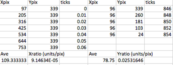
Table 1. The pixel coordinates of the ticks for each axis was recorded. Using Xpix and Ypix values, the ratios that convert image pixel coordinates to real x and y values were derived.
The conversion equations from pixel coordinates to the real coordinates are given by:
X = Xratio*(Xpix-97)
Y = Yratio*(Ypix-339)
The second and final task is to use the conversion ratios of x and y pixel coordinates to reconstruct the graph. The pixel coordinates of 5 data points from figure 1 are listed in a spreadsheet. Since the origins of the scanned plot and pixel coordinates are not at the same place, the x and y pixel coordinates of the original origin are subtracted from the data sets to offset the translation of one coordinate system with respect to the other. Finally, the x and y pixel values of each point are multiplied to the x and y conversion ratios. I therefore recovered the original x and y values of the data points. The reconstructed x and y values of the points are listed in table 2.
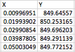
Table 2. Reconstructed data points. I derived the real x and y values of the data points based on their pixel coordinates.
I superimposed the scanned image and my plot in figure 2 and it turned out that they are very similar. Thus, I successfully reconstructed the original plot by carefully implementing the steps given by my instructor. For this activity, I rate myself as 9 since my plot resembles the original one.
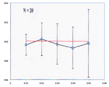 Figure 2. Superimposed image and reconstructed plot.
Acknowledgement
I would like to thank Ms. Krizzia Mañago for reviewing my work.
References:
[1] J.E. Tio. Simulation of a One Dimensional Photonic Crystal with Defects. October 2001.
[2] M. Soriano, Applied Physics 186 A2 – Digital Scanning. 2016.
