Scilab, like Matlab, is a coding platform that caters efficient matrix handling. The good thing about it is the fact that it is free! Its basic operations are very straightforward – matrix addition and multiplication are as simple as A + B and A*B. Useful for image processing, its procedures are mostly matrix manipulation.
Digital masking is an important tool in learning the basics of image processing and optical simulations. This is done by an element-by-element multiplication of the image and the mask.
For this activity, we are asked to generate 7 different synthetic images: square, sinusoid and grating along x direction, annulus, circular aperture with gaussian transparency, ellipse and cross. Each of them is generated by different functions which I will discuss in detail on the following sections.
The algorithm is basically divided into 3 parts: generation of a 2D grid, implementation of the generating function of the desired synthetic image and visualization of the image. Consider the algorithm for generating a square aperture provided in Figure 1. Line 1 closes all current Scilab figures. Since Scilab does not automatically close all the figures when executing another script, this line does the cleaning job. Lines 2-6 create an nx by ny 2D grid. Lines 7-12 are the implementation parts where the square image is generated. Note that I used A.*A1 in lines 14 and 17 to produce a square. A square is therefore basically done by an element-by-element multiplication of two orthogonal bars with the same thickness. The visualization of this process is given in figure. 2.a-2.c. The surface profile of the square is given in figure 2.d.
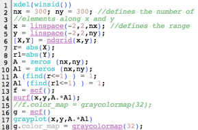 Figure 1. Code snippet for square aperture.
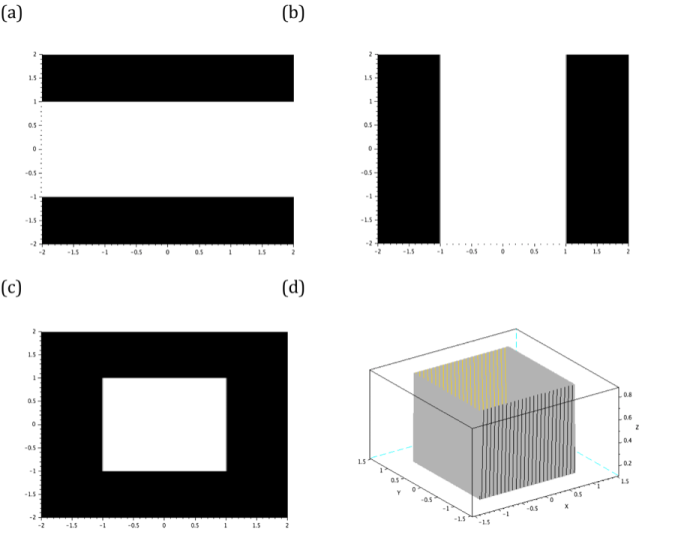
Figure 2. The element-by-element multiplication of (a) and (b) results to a square aperture (c). The profile of this aperture is given in (d).
The next synthetic image is a sinusoid. I generated it by taking the sine of the Y grid. The function is given by:
r=sin(nπY) (1)
The equation above replaces the generating function of square aperture. The variable n of equation 1 dictates the number of cycles in the sinusoid image. Note that the Y grid is used because the sinusoid must be along the X direction. The code and generated image are given in figures 3 and 4.
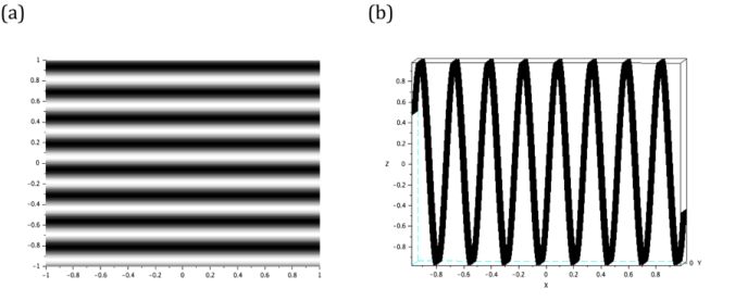 Figure 4. The siusoidal image is generated by taking the sine of Y grid. Its line scan is also given to visualize the profile of the image.
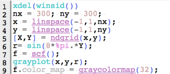 Figure 3. Code snippet for sinusoid image.
The binarization of the sinusoid image results to a grating. Using the same code given in figure 3, together with the binarization process, the achieved grating is presented in figure 5.
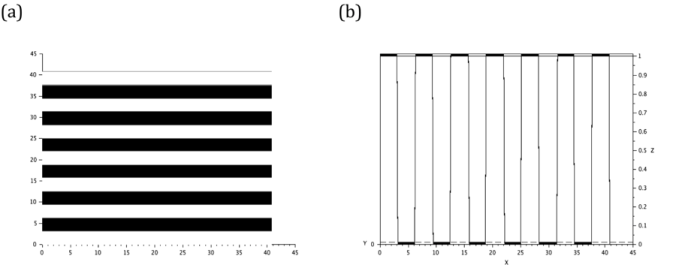 Figure 5. The binarization of the sinusoid in previous selections yields a grating (a). The profile (b) of the image is also given.
Annulus and circular masks are generated by the same function which is the equation of circle itself r= sqrt(X.^2 + Y.^2). However, the annulus is supposed to be hollow in the inside so I added a condition A (find(r<0.4)) = 0 wherein I punctured a a circle inside the bigger circle. The inner radius of the annulus is equal to the radius of the punctured area. The code snippet and the annulus mask are presented in figures 6 and 7.
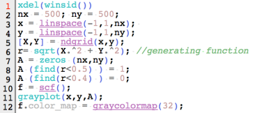 Figure 6. Code snippet for annulus.
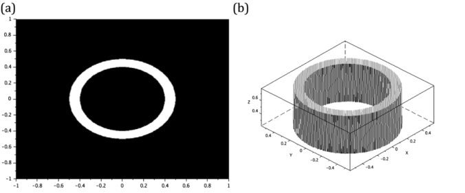 Figure 7. The annulus (a) generated has an outer and inner radii of 0.5 and 0.4 respectively. It profile is given in (b).
For the image of the ellipse, the function in equation 2 is implemented. First, set the right hand side of the equation 2 to an arbitrary variable r. Then, set all the points enclosed by the curve r into 1. These processes are shown in lines 6 and 9 from the algorithm in figure 8. The lengths of major and minor axes of the ellipse are designated to variables Ma and ma, respectively. The obtained elliptical synthetic image and its surface profile are presented in figure 9.
X^2/a^2 +Y^2/b^2 =1 (2)
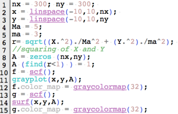 Figure 8. Code snippet for ellipse image.
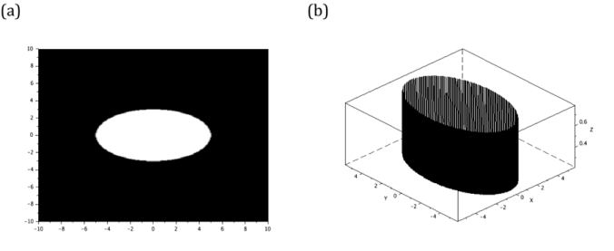 Figure 9. The generated ellipse (a), with major and minor axis lengths of 5 and 3 units respectively, and its profile (b) are shown here.
The next image is a cross. I visualize it as a superposition of two orthogonal rectangles. The generation of a rectangular aperture is similar to the process of creating a square aperture but the side lengths are not equal for this case. Lines 11-18 of figure 10 create two perpendicular rectangles. Line 19, on the other hand, superimposes the rectangles. Therefore, this shows that I can use matrix addition and element-by-element multiplication simultaneously to create my desired image. However, adding the two rectangles means that the intersection of their areas has more irradiance compared to the lateral parts of the cross. Using the lines 19-27, I smoothen the profile of the cross image by equating all the gray values inside the image to 1. The image and profile of the cross are both given in figure 11.
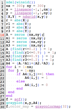 Figure 10. Code snippet for cross
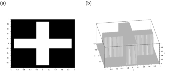 Figure 11. The cross (a) is generated by adding two orthogonal 1.8 x 0.4rectangles. Its profile is also given here (b).
The final image is a gaussian mask. It is known to blur the image impinged to it. [3] Its equation is given by:
G(x)= a*exp((-(x-b)^2)/(2c^2 )) (3)
where a is the peak value, b is the location of the center and c is the standard deviation. It is used as the generating function of the image.
The irradiance of gaussian mask image is concentrated inside the standard deviation (c). Hence, when another image is masked by a gaussian mask, the center detail remains clear as long as it is inside the radius equal to c. The remaining parts of the image inside this radius are blurred. The gaussian mask and its profile are presented in figure 13.
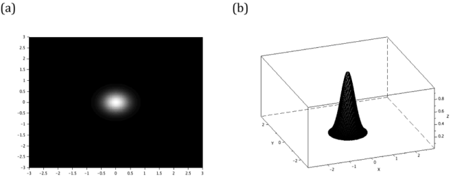 Figure 13. The gaussian mask (a) and its profile (b).
To sum up, I generated all the 7 images using some matrix manipulations available in Scilab. Hence, I give myself a score of 8. I think that some of my codes are lengthy even though I only performed all the steps that Dr. Soriano asked me to do.
Personally, I enjoy this activity because this teaches me how to make different apertures to play with light.
Acknowledgement:
I would like to thank Ms. Krizzia Mañago for reviewing my work and Ms. Niña Zambale for sharing her way of discussing this activity.
References:
[1] http://www.scilab.org/
[2] M. Soriano, Applied Physics 186 A3 – Scilab Basics. 2016
[3] http://homepages.inf.ed.ac.uk/rbf/HIPR2/gsmooth.htm
