Our next lesson is about Fourier transform wherein we transform some known functions from time to frequency domain. This is an interesting activity because here Fourier transform is applied to do simple image processing.
The first example is a circular aperture. The function fftshift is applied on the aperture to shift the quadrants. Fast Fourier transform algorithm, known as fft, assumes that the center of the object is indexed first. Therefore, there is a need to shift the quadrants such that they satisfies this assumption. Figure 1 shows the images of a circular aperture and its image when its 4 quadrants are shifted.
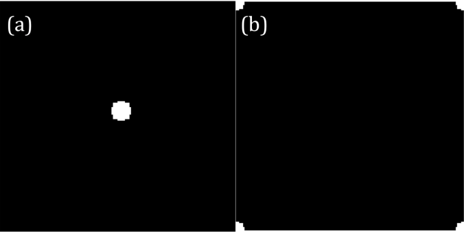
Figure 1. circular aperture (a) and its shifted version (b)
As I mentioned before, Fourier transform brings the image from time to frequency domain. In Fourier space, the values of each pixel are complex. To convince myself, I decomposed the transformed image into real and imaginary parts and I presented them in figure 2.b and 2.c. The pattern obtained when the magnitude of the transformed image is an airy pattern and it is showed in Figure 2.a. Cool! In some classes, we just derive the Fourier transform of some functions but here, we visualize it. I also did this to the Fourier transform of image “A” and the results are in Figure 3.
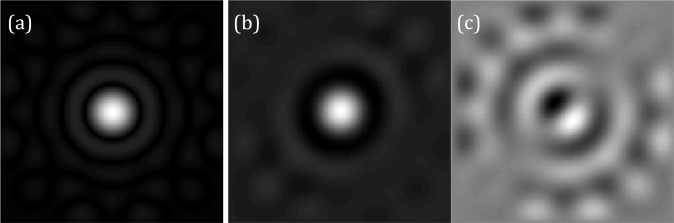
Figure 2. The Fourier transform of circle (a) is composed of real (b) and imaginary parts (c).
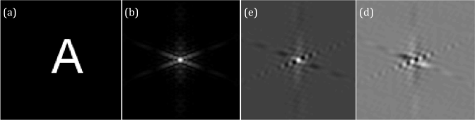
Figure 3. Image of letter “A” (a) and its Fourier transform (b). The transform is further decomposed into its real (e) and imaginary (d) components.
After the circle, I proceeded with corrugated roof, double slit, square function and Gaussian curve. For me, the corrugated roof is the best example to discuss Fourier transform to starters. Fourier transform follows the superposition principle where it is stated that all signals are sums sinusoids with different frequencies and amplitude modulation. A corrugated roof is basically a single sinusoid signal with one constant frequency. Its Fourier transform has 2 peaks equidistant from the origin located on the +/- frequency value as shown in figure 6b. It is a concrete visualization of what the Fourier transform really does to the input signal: it decomposes the input into its frequency components. Another interesting result is the fft of the double slit because it resembles the diffraction pattern of a double slit. This shows that I can also use fft to visualize the diffraction pattern of a given slit. The diffraction pattern of a square aperture also looks the same as its fft which is a sinc function. I displayed the corrugated roof, double slit and square aperture and their Fourier transforms in Figures 4-6.
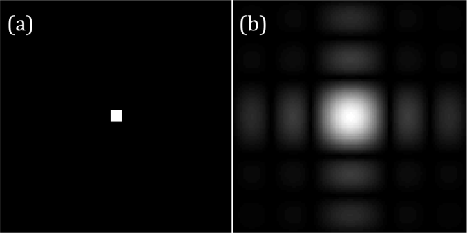
Figure 4. Square aperture (a) and its Fourier transform (b)
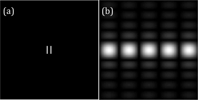
Figure 5. Double slit (a) and its Fourier transform (b)
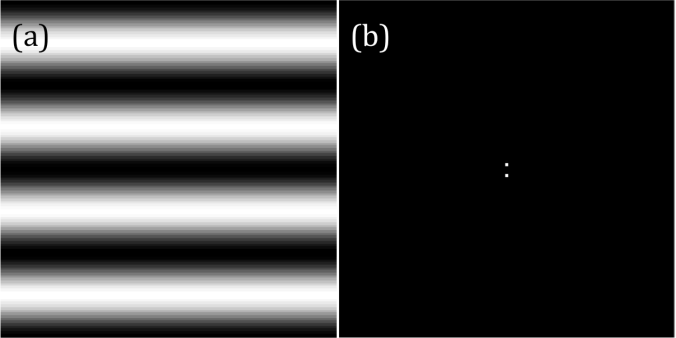
Figure 6. Corrugated roof along x-axis(a) and its Fourier transform (b)
Circular and square aperture, corrugated roof and double slit have some cool fft but the Gaussian aperture is different. The FFT of a Gaussian curve is still a Gaussian curve. Pretty boring isn’t it? But imagine this, if you have Gaussian beam and you propagate it to some distance you will still get a Gaussian beam! Most of the time, laser people wants their laser beam to have a same profile after propagating it at some distance. The Gaussian aperture and its Fourier transform is given in figure 7.
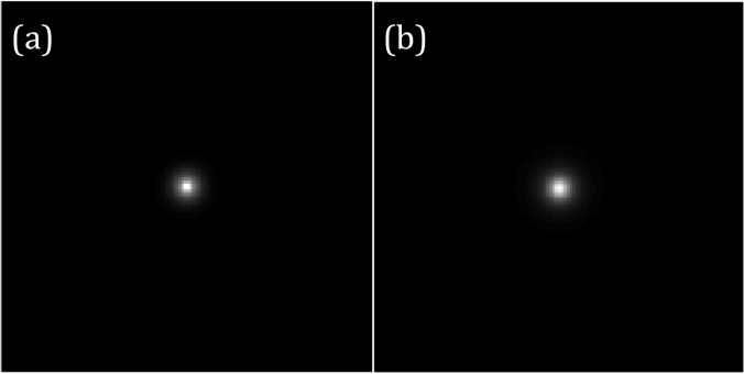
Figure 7. Gaussian aperture (a) and its Fourier transform (b)
The next basic concept is convolution. It is a systematic process of combining two signals. Convolution simulates the effects of the imaging systems to the final image registered in the camera sensor. For this section, I used an image of the word “VIP” and it is shown in figure 8d. Due to the finite diameter of the lens, only part of the information of the object is attainable for every imaging system. This is where convolution will come in. I convolved circular apertures with different radii to the 2D Fourier transform of the image to simulate the effect of the finite radius of the lens. The results are presented in figures 8d-e. As the size of the circular aperture becomes smaller, lesser frequencies are brought back to the time domain by inverse Fourier transform therefore the image becomes more and more blurred.
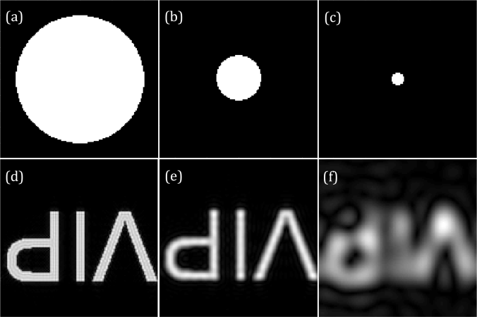
Figure 8. Imaging with different aperture size. Aperture in (a) yields the most slear ‘VIP’ image. The quality of the image degrades as the aperture becomes smaller.
Another image processing technique is the use of correlation to template matching. Here, I use an sentence and letter “A” rendered as images. The goal is to find where the A’s are in the sentence. Both of the images are transformed to Fourier space. The conjugate of the transformed image of the sentence is multiplied to the transformed image of “A”. The result is presented in Figure 9 and it shows that the intensity on the position of A’s in the sentence is higher compared to the rest of the letters.

Figure 9. The given pattern (a) is convolved with a template (b) to find the location of the template along the pattern. The bright peaks in (c) pinpoint the location of the template.
For the last part, Convolution is used for edge detection. Using the same “VIP” image and 3×3 matrices with total sum of 0, the vertical and horizontal edges are erased as shown in figure 10. The 3×3 matrices are, a = [-1 -1 -1; 2 2 2;-1 -1 -1], b = [-1 2 -1; -1 2 -1;-1 2 -1], and c = [-1 -1 -1; -1 8 -1; -1 -1 -1] . The edge detected by convolving the “VIP” image to either of the zero sum matrices given is perpendicular to the orientation of the arrays of -1’s from the matrix. The matrix a, for example, detects vertical edges.
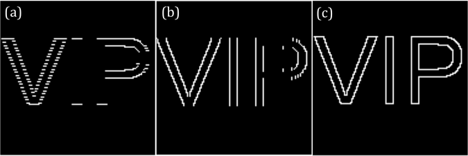
Figure 10. Edge detection using different 3×3 zero sum matrix.
Although this is an introductory activity, it took me a lot of time before I finished it. It is because I want to savor this topic. I would rate myself as 10.
Acknowledgement:
I would like to thank Ms. Krizzia Mañago for reviewing my work.
Reference:
[1] M. Soriano, AP 186 A5 – Fourier Transformation Model of Image Formation. 2016
[2] Smith, Ph.D. By Steven W. “The Scientist and Engineer’s Guide ToDigital Signal ProcessingBy Steven W. Smith, Ph.D.” Convolution. N.p., n.d. Web. 12Oct. 2016. http://www.dspguide.com/ch6.htm
